

178
16. Lattice Field Theory, and the Renormalization Group Revisited
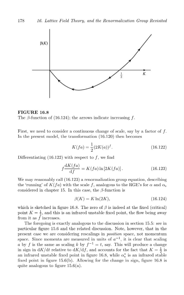
FIGURE 16.8
The β-function of (16.124); the arrows indicate increasing f .
First, we need to consider a continuous change of scale, say by a factor of f .
In the present model, the transformation (16.120) then becomes
K(f a) =
1
2
(2K(a))
f .
(16.122)
Differentiating (16.122) with respect to f , we find
f
dK(f a)
df
= K(f a) ln [2K(f a)] .
(16.123)
We may reasonably call (16.123) a renormalization group equation, describing
the ‘running’ of K(f a) with the scale f , analogous to the RGE’s for α and α s
considered in chapter 15. In this case, the β-function is
β(K) = K ln(2K),
(16.124)
which is sketched in figure 16.8. The zero of β is indeed at the fixed (critical)
1
point K = 2 , and this is an infrared unstable fixed point, the flow being away
from it as f increases.
The foregoing is exactly analogous to the discussion in section 15.5: see in
particular figure 15.6 and the related discussion. Note, however, that in the
present case we are considering rescalings in position space, not momentum
space. Since momenta are measured in units of a
−1 , it is clear that scaling
a by f is the same as scaling k by f
−1 = t, say. This will produce a change
1
in sign in dK/dt relative to dK/df , and accounts for the fact that K = is
2
an infrared unstable fixed point in figure 16.8, while α
∗ is an infrared stable
s
fixed point in figure 15.6(b). Allowing for the change in sign, figure 16.8 is
quite analogous to figure 15.6(a).