16.4. Renormalization, and the renormalization group, on the lattice
177
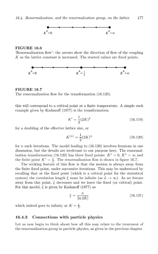
FIGURE 16.6
‘Renormalization flow’: the arrows show the direction of flow of the coupling
K as the lattice constant is increased. The starred values are fixed points.
FIGURE 16.7
The renormalization flow for the transformation (16.120).
this will correspond to a critical point at a finite temperature. A simple such
example given by Kadanoff (1977) is the transformation
′
K =
1 (2K)
2
(16.119)
2
for a doubling of the effective lattice size, or
1
K
(n) = (2K)
n
(16.120)
2
for n such iterations. The model leading to (16.120) involves fermions in one
dimension, but the details are irrelevant to our purpose here. The renormalization transformation (16.120) has three fixed points: K
∗ = 0, K
∗ = ∞ and
1
the finite point K
∗ = . The renormalization flow is shown in figure 16.7.
2
The striking feature of this flow is that the motion is always away from
the finite fixed point, under successive iterations. This may be understood by
recalling that at the fixed point (which is a critical point for the statistical
system) the correlation length ξ must be infinite (as L → ∞). As we iterate
away from this point, ξ decreases and we leave the fixed (or critical) point.
For this model, ξ is given by Kadanoff (1977) as
a
ξ =
(16.121)
|ln 2K|
1
which indeed goes to infinity at K = 2 .
16.4.3 Connections with particle physics
Let us now begin to think about how all this may relate to the treatment of
the renormalization group in particle physics, as given in the previous chapter.