16.4. Renormalization, and the renormalization group, on the lattice
175
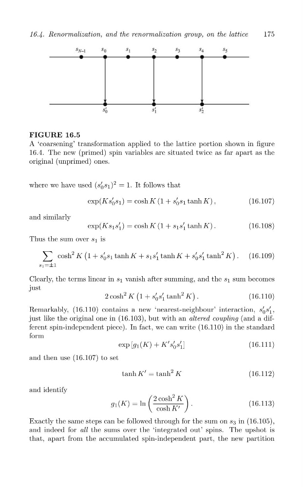
FIGURE 16.5
A ‘coarsening’ transformation applied to the lattice portion shown in figure
16.4. The new (primed) spin variables are situated twice as far apart as the
original (unprimed) ones.
′
where we have used (s 0 s 1 )
2 = 1. It follows that
′
′
exp(Ks 0 s 1 ) = cosh K (1 + s 0 s 1 tanh K) ,
(16.107)
and similarly
′
′
exp(Ks 1 s 1 ) = cosh K (1 + s 1 s 1 tanh K) .
(16.108)
Thus the sum over s 1 is
∑
(
)
′
′
′ ′
cosh
2 K 1 + s 0 s 1 tanh K + s 1 s 1 tanh K + s 0 s 1 tanh
2 K . (16.109)
s1 =±1
Clearly, the terms linear in s 1 vanish after summing, and the s 1 sum becomes
just
(
)
′ ′
2 cosh
2 K 1 + s 0 s 1 tanh
2 K .
(16.110)
′ ′
Remarkably, (16.110) contains a new ‘nearest-neighbour’ interaction, s 0 s 1 ,
just like the original one in (16.103), but with an altered coupling (and a different spin-independent piece). In fact, we can write (16.110) in the standard
form
′ ′
exp [g 1 (K) + K
′ s 0 s 1 ]
(16.111)
and then use (16.107) to set
tanh K
′ = tanh
2 K
(16.112)
and identify
(
)
2 cosh
2 K
g 1 (K) = ln
.
(16.113)
cosh K ′
Exactly the same steps can be followed through for the sum on s 3 in (16.105),
and indeed for all the sums over the ‘integrated out’ spins. The upshot is
that, apart from the accumulated spin-independent part, the new partition