

174
16. Lattice Field Theory, and the Renormalization Group Revisited
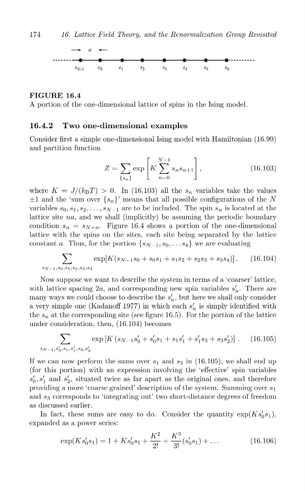
FIGURE 16.4
A portion of the one-dimensional lattice of spins in the Ising model.
16.4.2 Two one-dimensional examples
Consider first a simple one-dimensional Ising model with Hamiltonian (16.99)
and partition function
[
]
∑
N ∑ −1
Z =
exp K
s n s n+1 ,
(16.103)
{sn}
n=0
where K = J/(k B T ) > 0. In (16.103) all the s n variables take the values
±1 and the ‘sum over {s n }’ means that all possible configurations of the N
variables s 0 , s 1 , s 2 , . . . , s N −1 are to be included. The spin s n is located at the
lattice site na, and we shall (implicitly) be assuming the periodic boundary
condition s n = s N +n . Figure 16.4 shows a portion of the one-dimensional
lattice with the spins on the sites, each site being separated by the lattice
constant a. Thus, for the portion {s N 1 , s 0 , . . . s
−
4 } we are evaluating
∑
exp[K(s N 1 s 0 + s 0 s 1 + s 1 s +
−
2
s 2 s 3 + s 3 s 4 )] .
(16.104)
sN 1,s0 ,s1,s2,s3,s
−
4
Now suppose we want to describe the system in terms of a ‘coarser’ lattice,
with lattice spacing 2a, and corresponding new spin variables s
′
n . There are
many ways we could choose to describe the s
′
n , but here we shall only consider
a very simple one (Kadanoff 1977) in which each s
′
n is simply identified with
the s n at the corresponding site (see figure 16.5). For the portion of the lattice
under consideration, then, (16.104) becomes
∑
exp [K (s N 1 s 0
′ + s
′
0 s 1 + s 1 s 1
′ + s 1
′ s 3 + s
−
3 s
′
2 )] . (16.105)
sN
,s ,s ′
−1,s 0
′ ,s1,s ′
1 3 2
If we can now perform the sums over s 1 and s 3 in (16.105), we shall end up
(for this portion) with an expression involving the ‘effective’ spin variables
s
′
0 , s
′
1 and s
′
2 , situated twice as far apart as the original ones, and therefore
providing a more ‘coarse grained’ description of the system. Summing over s 1
and s 3 corresponds to ‘integrating out’ two short-distance degrees of freedom
as discussed earlier.
In fact, these sums are easy to do. Consider the quantity exp(Ks
′
0 s 1 ),
expanded as a power series:
K
2
K
3
exp(Ks
′
0 s 1 ) = 1 + Ks
′
0 s 1 +
+
(s
′ s 1 ) + . . .
(16.106)
2!
3!
0