

16.3. Representation of quantum amplitudes
161
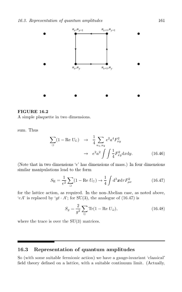
FIGURE 16.2
A simple plaquette in two dimensions.
sum. Thus
∑
1 ∑
(1 − Re U
2
❗ ) →
e
2 a
4 F
4
xy
❗
n1,n
∫ ∫
2
→ e
2 a
2
1 F
2
xy dxdy.
(16.46)
4
(Note that in two dimensions ‘e’ has dimensions of mass.) In four dimensions
similar manipulations lead to the form
∫
1 ∑
1
S =
(1 − Re U ) →
d
3
2
E
❗
xdτF
(16.47)
e 2
4
μν
❗
for the lattice action, as required. In the non-Abelian case, as noted above,
‘eA’ is replaced by ‘gt · A’; for SU(3), the analogue of (16.47) is
2 ∑
S g =
Tr(1
g 2
❗
− Re U ❗ ),
(16.48)
where the trace is over the SU(3) matrices.
16.3 Representation of quantum amplitudes
So (with some suitable fermionic action) we have a gauge-invariant ‘classical’
field theory defined on a lattice, with a suitable continuum limit. (Actually,