160
16. Lattice Field Theory, and the Renormalization Group Revisited
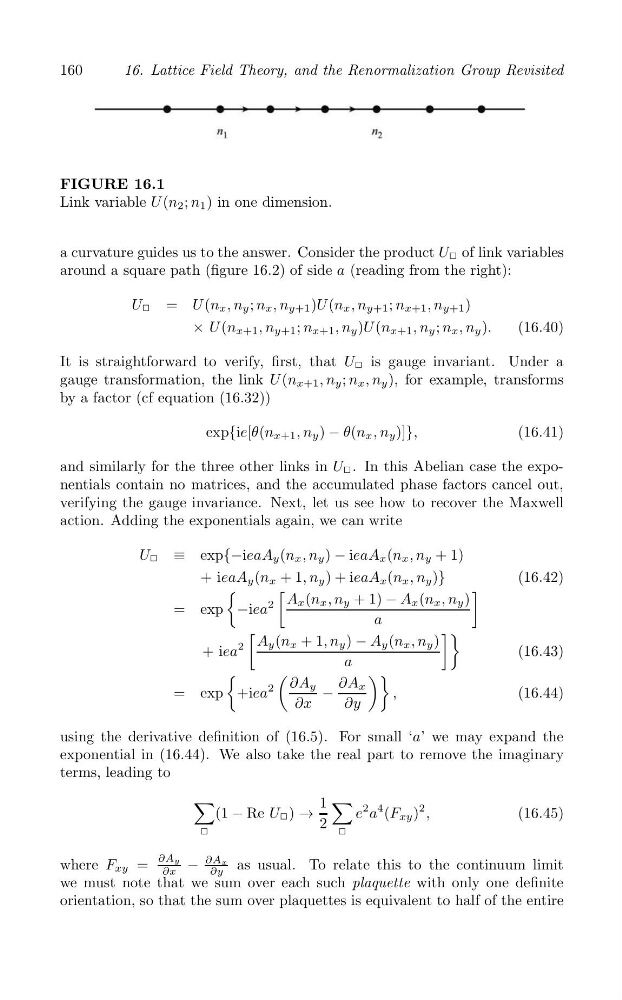
FIGURE 16.1
Link variable U (n 2 ; n 1 ) in one dimension.
a curvature guides us to the answer. Consider the product U ❗ of link variables
around a square path (figure 16.2) of side a (reading from the right):
U ❗ = U (n x , n y ; n x , n y+1 )U (n x , n y+1 ; n x+1 , n y+1 )
× U (n x+1 , n y+1 ; n x+1 , n y )U (n x+1 , n y ; n x , n y ).
(16.40)
It is straightforward to verify, first, that U ❗ is gauge invariant. Under a
gauge transformation, the link U (n x+1 , n y ; n x , n y ), for example, transforms
by a factor (cf equation (16.32))
exp{ie[θ(n x+1 , n y ) − θ(n x , n y )]},
(16.41)
and similarly for the three other links in U ❗ . In this Abelian case the exponentials contain no matrices, and the accumulated phase factors cancel out,
verifying the gauge invariance. Next, let us see how to recover the Maxwell
action. Adding the exponentials again, we can write
U ❗ ≡ exp{−ieaA y (n x , n y ) − ieaA x (n x , n y + 1)
+ ieaA y (n x + 1, n y ) + ieaA x (n x , n y )}
(16.42)
(
[
]
A x (n x , n y + 1) − A x (n x , n y )
2
= exp
−iea
a
[
])
A y (n x + 1, n y ) − A y (n x , n y )
2
+ iea
(16.43)
a
(
(
))
∂A y
∂A x
2
= exp
+iea
−
,
(16.44)
∂x
∂y
using the derivative definition of (16.5). For small ‘a’ we may expand the
exponential in (16.44). We also take the real part to remove the imaginary
terms, leading to
∑
∑
1
2
(1 − Re U ❗ ) →
e a
4 (F xy )
2 ,
(16.45)
2
❗
❗
∂Ay −
∂Ax
where F xy =
as usual. To relate this to the continuum limit
∂x
∂y
we must note that we sum over each such plaquette with only one definite
orientation, so that the sum over plaquettes is equivalent to half of the entire