16.2. Discretization
155
a form suitable for numerical simulation, which we defer until section 16.3.
There is, however, a quite separate problem which arises when we try to repeat
for the Dirac field the discretization used for the scalar field.
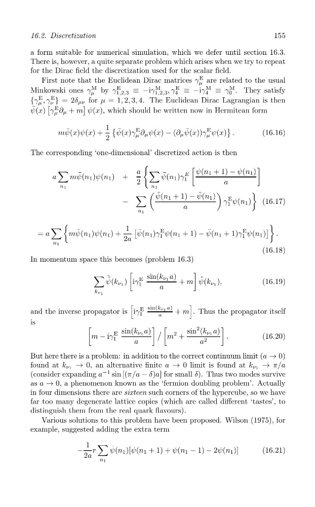
First note that the Euclidean Dirac matrices γ
E
μ are related to the usual
Minkowski ones γ
M
μ by γ
E
1,2,3 ≡ −iγ
M
E
M
M
1,2,3 , γ 4 ≡ −iγ 4 ≡ γ 0 . They satisfy
{γ
E
μ , γ
E
[ ν } = 2δ μν ]
for μ = 1, 2, 3, 4. The Euclidean Dirac Lagrangian is then
¯
ψ(x) γ
E
μ ∂ μ + m ψ(x), which should be written now in Hermitean form
1 {
}
¯
¯
¯
mψ(x)ψ(x) +
ψ(x)γ
E
μ ∂ μ ψ(x) − (∂ μ ψ(x))γ
E
μ ψ(x) .
(16.16)
2
The corresponding ‘one-dimensional’ discretized action is then
(
[
]
∑
a ∑
E ψ(n 1 + 1) ψ(n )
¯
¯
1
a
mψ(n 1 )ψ(n 1 ) +
ψ(n 1 )γ
−
2
1
a
n1
(
n1
)
)
∑ ¯
ψ(n
−
1 + 1) − ¯
ψ(n 1 ) γ
E
a
1 ψ(n 1 ) (16.17)
n1
(
)
∑
1 [
]
¯
¯
¯
= a
mψ(n 1 )ψ(n 1 ) +
ψ(n 1 )γ
E
1 ψ(n 1 + 1) − ψ(n 1 + 1)γ
E
1 ψ(n 1 ) .
2a
n1
(16.18)
In momentum space this becomes (problem 16.3)
[
]
∑ ¯
sin(k ν a)
˜
˜
ψ(k ν1 ) iγ
E
1
1
+ m ψ(k ν ,
(16.
a
1 )
19)
kν 1
[
]
sin(k a)
and the inverse propagator is iγ
E
ν 1
1
+ m . Thus the propagator itself
a
is
[
] [
]
m − iγ
E sin(k ν1 a) /
ν
m
2
sin
2 (k
+
1 a)
1
.
(16.20)
a
a 2
But here there is a problem: in addition to the correct continuum limit (a → 0)
found at k ν1 → 0, an alternative finite a → 0 limit is found at k ν1 → π/a
(consider expanding a
−1 sin [(π/a − δ)a] for small δ). Thus two modes survive
as a → 0, a phenomenon known as the ‘fermion doubling problem’. Actually
in four dimensions there are sixteen such corners of the hypercube, so we have
far too many degenerate lattice copies (which are called different ‘tastes’, to
distinguish them from the real quark flavours).
Various solutions to this problem have been proposed. Wilson (1975), for
example, suggested adding the extra term
1 ∑
−
¯
r
ψ(n 1 )[ψ(n 1 + 1) + ψ(n 1
21)
2a
1
− 1) − 2ψ(n 1 )]
(16.
n