154
16. Lattice Field Theory, and the Renormalization Group Revisited
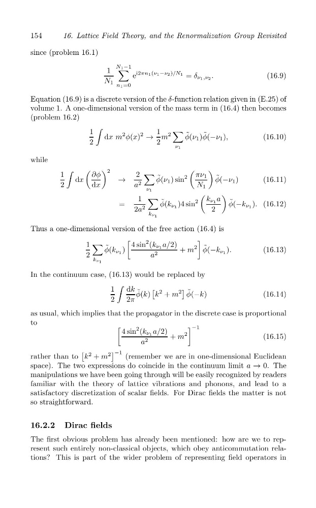
since (problem 16.1)
N 1
1 ∑ 1−
e
i2πn1(ν1−ν2)/N1 = δ ν ,ν .
(16.9)
N
1 2
1 n1=0
Equation (16.9) is a discrete version of the δ-function relation given in (E.25) of
volume 1. A one-dimensional version of the mass term in (16.4) then becomes
(problem 16.2)
∫
1
˜
dx m
2
1
∑
(x)
2
→
˜
φ
m
2
φ(ν 1 )φ( 1 ,
2
ν
−ν )
(16.10)
2
1
while
∫
( ) 2
(
)
1
∂φ
2 ∑
d
n
2
πν
˜
x
→
˜
1
φ(ν 1 ) si
φ(
(
2
dx
a 2
N
ν1
−ν 1 )
16.11)
1
(
)
1 ∑
k ν a
˜
=
φ(k
2
1
˜
ν1 )4 sin
φ(
2a 2
2
k
−k ν1 ). (16.12)
ν 1
Thus a one-dimensional version of the free action (16.4) is
[
1 ∑
n
2
]
4 si (k
˜
ν a/2)
˜
φ(k 1 )
1
ν
+ m
2 φ(
2
a 2
k
−k ν1 ).
(16.13)
ν 1
In the continuum case, (16.13) would be replaced by
∫
1
dk
[
]
˜
φ(k) k
2 + m
2 ˜
φ(
2
2π
−k)
(16.14)
as usual, which implies that the propagator in the discrete case is proportional
to
[
4 sin
2
]
(k ν a/2)
−1
1
+ m
2
(16.15)
a 2
[
]
rather than to k
2 + m
2 −1 (remember we are in one-dimensional Euclidean
space). The two expressions do coincide in the continuum limit a → 0. The
manipulations we have been going through will be easily recognized by readers
familiar with the theory of lattice vibrations and phonons, and lead to a
satisfactory discretization of scalar fields. For Dirac fields the matter is not
so straightforward.
16.2.2 Dirac fields
The first obvious problem has already been mentioned: how are we to represent such entirely non-classical objects, which obey anticommutation relations? This is part of the wider problem of representing field operators in