

120
15. QCD II: Asymptotic Freedom, the Renormalization Group
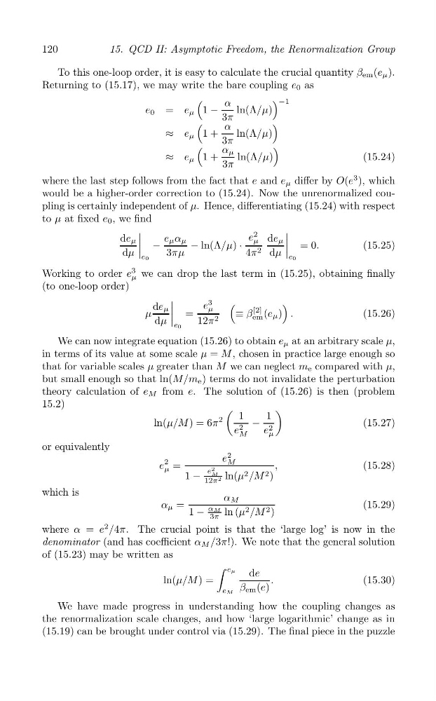
To this one-loop order, it is easy to calculate the crucial quantity β em (e μ ).
Returning to (15.17), we may write the bare coupling e 0 as
(
) −1
α
e 0 = e μ 1 −
ln(Λ/μ)
3π
(
)
α
≈ e μ 1 +
ln(Λ/μ)
3π
(
)
α μ
≈ e μ 1 +
ln(Λ/μ)
(15.24)
3π
where the last step follows from the fact that e and e μ differ by O(e
3 ), which
would be a higher-order correction to (15.24). Now the unrenormalized coupling is certainly independent of μ. Hence, differentiating (15.24) with respect
to μ at fixed e 0 , we find
de μ
e μ α μ
e μ
2 de μ
−
− ln(Λ/μ) ·
= 0.
(15.25)
dμ
|
|
|
|
3πμ
4π 2 dμ
|
|
|
|
e0
e0
3
Working to order e we can drop the last term in (15.25), obtaining finally
μ
(to one-loop order)
|
3
(
)
e
de μ
μ
≡ β
[2]
μ
=
(e μ ) .
(15.26)
|
|
|
em
dμ
12π 2
e0
We can now integrate equation (15.26) to obtain e μ at an arbitrary scale μ,
in terms of its value at some scale μ = M , chosen in practice large enough so
that for variable scales μ greater than M we can neglect m e compared with μ,
but small enough so that ln(M/m e ) terms do not invalidate the perturbation
theory calculation of e M from e. The solution of (15.26) is then (problem
15.2)
(
)
ln(μ/M ) = 6π
2
1 −
1
(15.27)
e 2
e 2
M
μ
or equivalently
2
e
e
2 =
2
M
,
(15.28)
μ
e
1 −
M ln(μ 2 /M 2 )
12π 2
which is
α M
α μ =
(15.29)
1 −
αM ln (μ 2 /M 2 )
3π
where α = e
2 /4π. The crucial point is that the ‘large log’ is now in the
denominator (and has coefficient α M /3π!). We note that the general solution
of (15.23) may be written as
∫ eμ de
ln(μ/M ) =
.
(15.30)
eM β em (e)
We have made progress in understanding how the coupling changes as
the renormalization scale changes, and how ‘large logarithmic’ change as in
(15.19) can be brought under control via (15.29). The final piece in the puzzle