

100
14. QCD I: Introduction, Tree Graph Predictions, and Jets
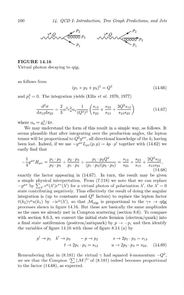
FIGURE 14.16
Virtual photon decaying to q¯ qg.
as follows from
(p 1 + p 2 + p 3 )
2 = Q
2
(14.66)
and p
2
i = 0. The integration yields (Ellis et al. 1976, 1977)
2
(
)
d σ
2
s 13
s 23
2 s
= α
2 e
2
1
Q
2
12
a α s
+
+
(14.67)
ds 13 ds
3
( 2 ) 3
23
Q
s 23
s 13
s 13 s 23
where α s = g
2
s /4π.
We may understand the form of this result in a simple way, as follows. It
seems plausible that after integrating over the production angles, the lepton
tensor will be proportional to Q
2 g
μν , all directional knowledge of the k i having
been lost. Indeed, if we use −g
μν L μν (p, p) = 4p · p
′ together with (14.62) we
easily find that
1
p
− g
μν
1 p 3
p 2 p 3
p 1 p 2 Q
2
s 13
s 23
2Q
2 s 12
H μν =
·
+
·
+
·
=
+
+
,
4
p 2 · p 3
p 1 · p 3
(p 1 · p 3 )(p 2 · p 3 )
s 23
s 13
s 13 s 23
(14.68)
exactly the factor appearing in (14.67). In turn, the result may be given
a simple physical interpretation. From (7.118) we note that we can replace
−g
μν by λ ∈
μ (λ
′ )∈
ν∗ (λ
′ ) for a virtual photon of polarization λ
′ , the λ
′
′ = 0
state contributing negatively. Thus effectively the result of doing the angular
integration is (up to constants and Q
2 factors) to replace the lepton factor
v ¯(k 2 )γ
μ u(k 1 ) by −i∈
μ (λ
′ ), so that M q¯ qg is proportional to the γ∗ → q¯ qg
processes shown in figure 14.16. But these are basically the same amplitudes
as the ones we already met in Compton scattering (section 8.6). To compare
with section 8.6.3, we convert the initial state fermion (electron/quark) into
a final state antifermion (positron/antiquark) by p → −p, and then identify
the variables of figure 14.16 with those of figure 8.14 (a) by
p
′
→ p 1 k
′
→ p 3
− p → p 2
s → 2p 1 · p 3 = s 13
t → 2p 1 · p 2 = s 12
u → 2p 2 · p 3 = s 23 . (14.69)
Remembering that in (8.181) the virtual γ had squared 4-momentum −Q
2 ,
we see that the Compton ‘ | M |
2 ’ of (8.181) indeed becomes proportional
to the factor (14.68), as expected.