

92
14. QCD I: Introduction, Tree Graph Predictions, and Jets
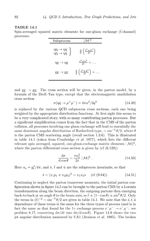
TABLE 14.1
Spin-averaged squared matrix elements for one-gluon exchange (t ˆ -channel)
processes.
Subprocess
|M|
2
)
(
)
qq
q¯ q
→ qq
4 s ˆ
2 +ˆ u
2
→ q¯ q
9
t ˆ2
s ˆ
2 +ˆ u
2
qg → qg
ˆ2
+ . . .
t
(
)
9 s ˆ
2 +ˆ u
2
gg → gg
4
t ˆ2
+ . . .
and gg → gg. The cross section will be given, in the parton model, by a
formula of the Drell–Yan type, except that the electromagnetic annihilation
cross section
σ(qq ¯ → μ
+ μ
− ) = 4πα
2 /3q
2
(14.49)
is replaced by the various QCD subprocess cross sections, each one being
weighted by the appropriate distribution functions. At first sight this seems to
be a very complicated story, with so many contributing parton processes. But
a significant simplification comes from the fact that in the CMS of the parton
collision, all processes involving one gluon exchange will lead to essentially the
same dominant angular distribution of Rutherford-type, ∼ sin
−4 θ/2, where θ
is the parton CMS scattering angle (recall section 1.3.6). This is illustrated
in table 14.1 (taken from Combridge et al. 1977), which lists the different
relevant spin averaged, squared, one-gluon-exchange matrix elements | M |
2 ,
where the parton differential cross section is given by (cf (6.129))
dσ
πα
2
=
s
2 .
(14.50)
d cos θ
2ˆ s
|M|
Here α s = g
2
ˆ
s /4π, and s ˆ, t and u ˆ are the subprocess invariants, so that
s ˆ = (x 1 p + x
2
1
2 p 2 ) = x 1 x 2 s (cf (9.84)).
(14.51)
Continuing to neglect the parton transverse momenta, the initial parton configuration shown in figure 14.5 can be brought to the parton CMS by a Lorentz
transformation along the beam direction, the outgoing partons then emerging
back-to-back at an angle θ to the beam axis, so t ˆ ∝ (1−cos θ) ∝ sin
2 θ/2. Only
the terms in (t ˆ )
−2
∼ sin
−4 θ/2 are given in table 14.1. We note that the s, ˆ t, ˆ u ˆ
dependence of these terms is the same for the three types of process (and is in
fact the same as that found for the 1γ exchange process e
− μ
−
→ e
− μ
− : see
problem 8.17, converting dσ/dt into dσ/d cos θ). Figure 14.9 shows the two
jet angular distribution measured by UA1 (Arnison et al. 1985). The broken
14. QCD I: Introduction, Tree Graph Predictions, and Jets
TABLE 14.1
Spin-averaged squared matrix elements for one-gluon exchange (t ˆ -channel)
processes.
Subprocess
|M|
2
)
(
)
q¯ q
4 s ˆ
2 +ˆ u
2
→ q¯ q
9
t ˆ2
s ˆ
2 +ˆ u
2
qg → qg
ˆ2
+ . . .
t
(
)
9 s ˆ
2 +ˆ u
2
gg → gg
4
t ˆ2
+ . . .
and gg → gg. The cross section will be given, in the parton model, by a
formula of the Drell–Yan type, except that the electromagnetic annihilation
cross section
σ(qq ¯ → μ
+ μ
− ) = 4πα
2 /3q
2
(14.49)
is replaced by the various QCD subprocess cross sections, each one being
weighted by the appropriate distribution functions. At first sight this seems to
be a very complicated story, with so many contributing parton processes. But
a significant simplification comes from the fact that in the CMS of the parton
collision, all processes involving one gluon exchange will lead to essentially the
same dominant angular distribution of Rutherford-type, ∼ sin
−4 θ/2, where θ
is the parton CMS scattering angle (recall section 1.3.6). This is illustrated
in table 14.1 (taken from Combridge et al. 1977), which lists the different
relevant spin averaged, squared, one-gluon-exchange matrix elements | M |
2 ,
where the parton differential cross section is given by (cf (6.129))
dσ
πα
2
=
s
2 .
(14.50)
d cos θ
2ˆ s
|M|
Here α s = g
2
ˆ
s /4π, and s ˆ, t and u ˆ are the subprocess invariants, so that
s ˆ = (x 1 p + x
2
1
2 p 2 ) = x 1 x 2 s (cf (9.84)).
(14.51)
Continuing to neglect the parton transverse momenta, the initial parton configuration shown in figure 14.5 can be brought to the parton CMS by a Lorentz
transformation along the beam direction, the outgoing partons then emerging
back-to-back at an angle θ to the beam axis, so t ˆ ∝ (1−cos θ) ∝ sin
2 θ/2. Only
the terms in (t ˆ )
−2
∼ sin
−4 θ/2 are given in table 14.1. We note that the s, ˆ t, ˆ u ˆ
dependence of these terms is the same for the three types of process (and is in
fact the same as that found for the 1γ exchange process e
− μ
−
→ e
− μ
− : see
problem 8.17, converting dσ/dt into dσ/d cos θ). Figure 14.9 shows the two
jet angular distribution measured by UA1 (Arnison et al. 1985). The broken