

82
14. QCD I: Introduction, Tree Graph Predictions, and Jets
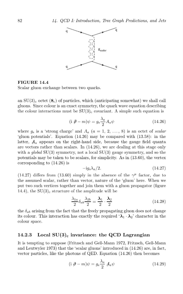
FIGURE 14.4
Scalar gluon exchange between two quarks.
an SU(3) c octet (8 c ) of particles, which (anticipating somewhat) we shall call
gluons. Since colour is an exact symmetry, the quark wave equation describing
the colour interactions must be SU(3) c covariant. A simple such equation is
λ a
(i / ∂ − m)ψ = g s A a ψ
(14.26)
2
where g s is a ‘strong charge’ and A a (a = 1, 2, . . . , 8) is an octet of scalar
‘gluon potentials’. Equation (14.26) may be compared with (13.58): in the
latter, / A a appears on the right-hand side, because the gauge field quanta
are vectors rather than scalars. In (14.26), we are dealing at this stage only
with a global SU(3) symmetry, not a local SU(3) gauge symmetry, and so the
potentials may be taken to be scalars, for simplicity. As in (13.60), the vertex
corresponding to (14.26) is
−ig s λ a /2.
(14.27)
(14.27) differs from (13.60) simply in the absence of the γ
μ factor, due to
the assumed scalar, rather than vector, nature of the ‘gluon’ here. When we
put two such vertices together and join them with a gluon propagator (figure
14.4), the SU(3) c structure of the amplitude will be
λ 1a
λ 2b
λ 1 λ 2
δ ab
=
·
(14.28)
2
2
2
2
the δ ab arising from the fact that the freely propagating gluon does not change
its colour. This interaction has exactly the required ‘λ 1 · λ 2 ’ character in the
colour space.
14.2.3 Local SU(3) c invariance: the QCD Lagrangian
It is tempting to suppose (Fritzsch and Gell-Mann 1972, Fritzsch, Gell-Mann
and Leutwyler 1973) that the ‘scalar gluons’ introduced in (14.26) are, in fact,
vector particles, like the photons of QED. Equation (14.26) then becomes
λ a
(i / ∂ − m)ψ = g s
A / a ψ
(14.29)
2
14. QCD I: Introduction, Tree Graph Predictions, and Jets
FIGURE 14.4
Scalar gluon exchange between two quarks.
an SU(3) c octet (8 c ) of particles, which (anticipating somewhat) we shall call
gluons. Since colour is an exact symmetry, the quark wave equation describing
the colour interactions must be SU(3) c covariant. A simple such equation is
λ a
(i / ∂ − m)ψ = g s A a ψ
(14.26)
2
where g s is a ‘strong charge’ and A a (a = 1, 2, . . . , 8) is an octet of scalar
‘gluon potentials’. Equation (14.26) may be compared with (13.58): in the
latter, / A a appears on the right-hand side, because the gauge field quanta
are vectors rather than scalars. In (14.26), we are dealing at this stage only
with a global SU(3) symmetry, not a local SU(3) gauge symmetry, and so the
potentials may be taken to be scalars, for simplicity. As in (13.60), the vertex
corresponding to (14.26) is
−ig s λ a /2.
(14.27)
(14.27) differs from (13.60) simply in the absence of the γ
μ factor, due to
the assumed scalar, rather than vector, nature of the ‘gluon’ here. When we
put two such vertices together and join them with a gluon propagator (figure
14.4), the SU(3) c structure of the amplitude will be
λ 1a
λ 2b
λ 1 λ 2
δ ab
=
·
(14.28)
2
2
2
2
the δ ab arising from the fact that the freely propagating gluon does not change
its colour. This interaction has exactly the required ‘λ 1 · λ 2 ’ character in the
colour space.
14.2.3 Local SU(3) c invariance: the QCD Lagrangian
It is tempting to suppose (Fritzsch and Gell-Mann 1972, Fritzsch, Gell-Mann
and Leutwyler 1973) that the ‘scalar gluons’ introduced in (14.26) are, in fact,
vector particles, like the photons of QED. Equation (14.26) then becomes
λ a
(i / ∂ − m)ψ = g s
A / a ψ
(14.29)
2