

52
13. Local Non-Abelian (Gauge) Symmetries
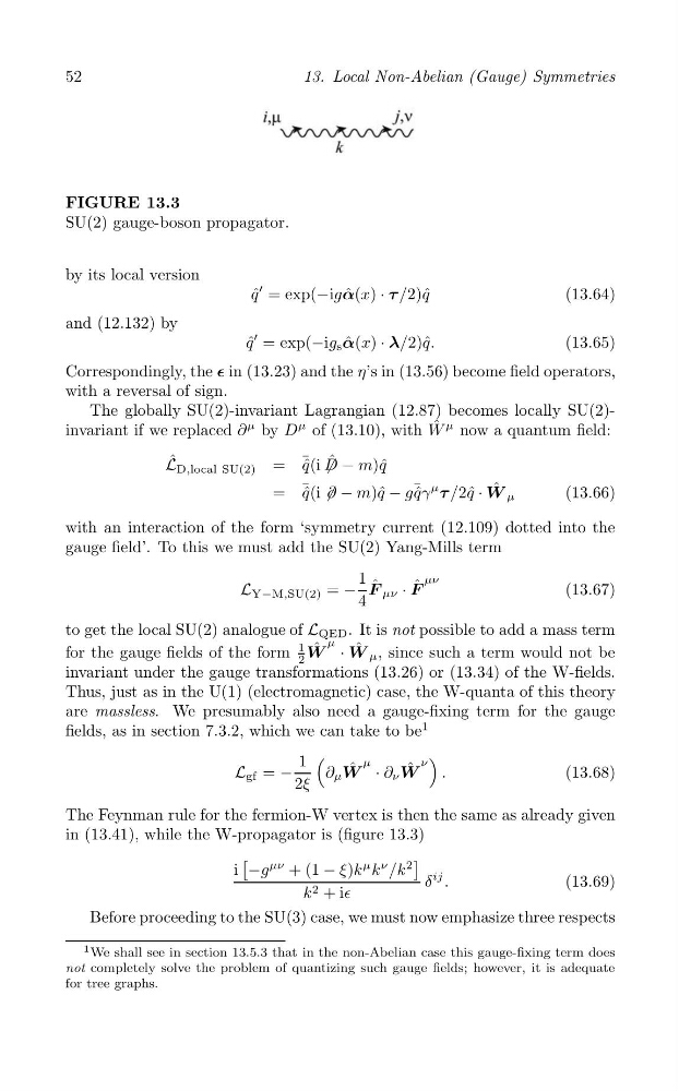
FIGURE 13.3
SU(2) gauge-boson propagator.
by its local version
′
q ˆ = exp(−igα ˆ (x) · τ /2)ˆ q
(13.64)
and (12.132) by
′
q ˆ = exp(−ig s α ˆ (x) · λ/2)ˆ q.
(13.65)
Correspondingly, the ∊ in (13.23) and the η’s in (13.56) become field operators,
with a reversal of sign.
The globally SU(2)-invariant Lagrangian (12.87) becomes locally SU(2)invariant if we replaced ∂
μ by D
μ of (13.10), with W ˆ μ now a quantum field:
ˆ
q(i D − m)ˆ
L ˆ D,local SU(2) = ¯ ˆ /
q
= ˆ /
m)ˆ
ˆ
q W μ
¯ q(i ∂ − q − g ¯ qγ
μ
τ /2ˆ · ˆ
(13.66)
with an interaction of the form ‘symmetry current (12.109) dotted into the
gauge field’. To this we must add the SU(2) Yang-Mills term
1
μν
L Y−M,SU(2) = − F ˆ μν · F ˆ
(13.67)
4
to get the local SU(2) analogue of L QED . It is not possible to add a mass term
μ
ˆ
ˆ
for the gauge fields of the form
1
W · W μ , since such a term would not be
2
invariant under the gauge transformations (13.26) or (13.34) of the W-fields.
Thus, just as in the U(1) (electromagnetic) case, the W-quanta of this theory
are massless. We presumably also need a gauge-fixing term for the gauge
fields, as in section 7.3.2, which we can take to be
1
(
)
1
μ
ν
ˆ
ˆ
L gf = −
∂ μ W · ∂ ν W .
(13.68)
2ξ
The Feynman rule for the fermion-W vertex is then the same as already given
in (13.41), while the W-propagator is (figure 13.3)
[
]
i −g
μν + (1 − ξ)k
μ k
ν /k
2
δ
ij .
(13.69)
k 2 + i∈
Before proceeding to the SU(3) case, we must now emphasize three respects
1 We shall see in section 13.5.3 that in the non-Abelian case this gauge-fixing term does
not completely solve the problem of quantizing such gauge fields; however, it is adequate
for tree graphs.
13. Local Non-Abelian (Gauge) Symmetries
FIGURE 13.3
SU(2) gauge-boson propagator.
by its local version
′
q ˆ = exp(−igα ˆ (x) · τ /2)ˆ q
(13.64)
and (12.132) by
′
q ˆ = exp(−ig s α ˆ (x) · λ/2)ˆ q.
(13.65)
Correspondingly, the ∊ in (13.23) and the η’s in (13.56) become field operators,
with a reversal of sign.
The globally SU(2)-invariant Lagrangian (12.87) becomes locally SU(2)invariant if we replaced ∂
μ by D
μ of (13.10), with W ˆ μ now a quantum field:
ˆ
q(i D − m)ˆ
L ˆ D,local SU(2) = ¯ ˆ /
q
= ˆ /
m)ˆ
ˆ
q W μ
¯ q(i ∂ − q − g ¯ qγ
μ
τ /2ˆ · ˆ
(13.66)
with an interaction of the form ‘symmetry current (12.109) dotted into the
gauge field’. To this we must add the SU(2) Yang-Mills term
1
μν
L Y−M,SU(2) = − F ˆ μν · F ˆ
(13.67)
4
to get the local SU(2) analogue of L QED . It is not possible to add a mass term
μ
ˆ
ˆ
for the gauge fields of the form
1
W · W μ , since such a term would not be
2
invariant under the gauge transformations (13.26) or (13.34) of the W-fields.
Thus, just as in the U(1) (electromagnetic) case, the W-quanta of this theory
are massless. We presumably also need a gauge-fixing term for the gauge
fields, as in section 7.3.2, which we can take to be
1
(
)
1
μ
ν
ˆ
ˆ
L gf = −
∂ μ W · ∂ ν W .
(13.68)
2ξ
The Feynman rule for the fermion-W vertex is then the same as already given
in (13.41), while the W-propagator is (figure 13.3)
[
]
i −g
μν + (1 − ξ)k
μ k
ν /k
2
δ
ij .
(13.69)
k 2 + i∈
Before proceeding to the SU(3) case, we must now emphasize three respects
1 We shall see in section 13.5.3 that in the non-Abelian case this gauge-fixing term does
not completely solve the problem of quantizing such gauge fields; however, it is adequate
for tree graphs.