

42
13. Local Non-Abelian (Gauge) Symmetries
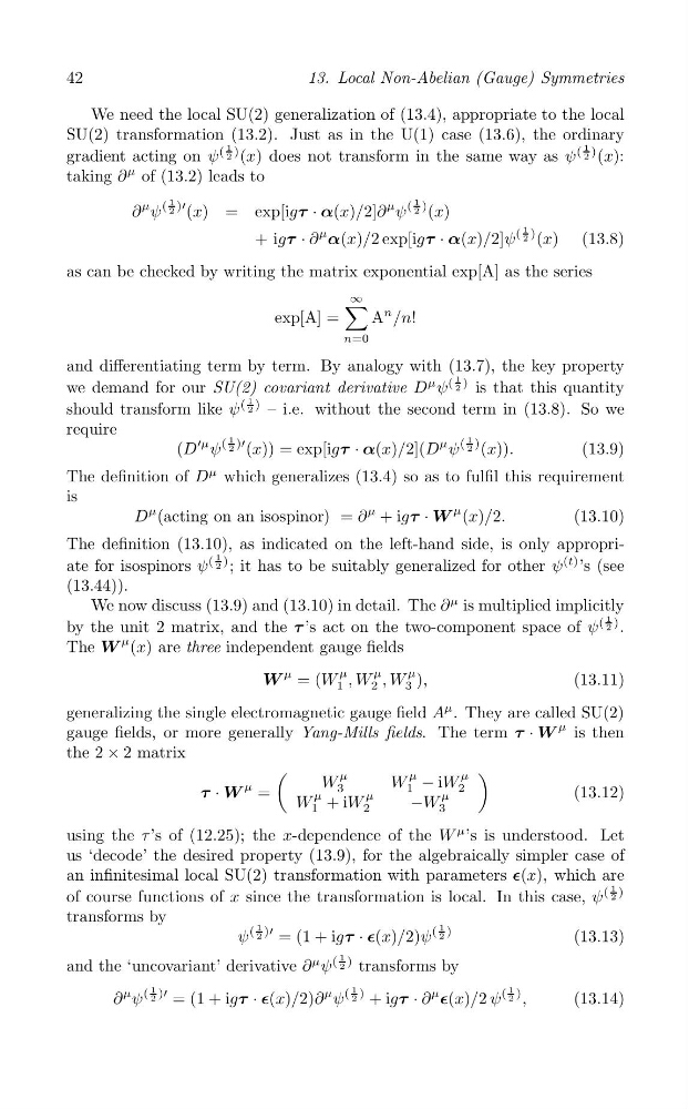
We need the local SU(2) generalization of (13.4), appropriate to the local
SU(2) transformation (13.2). Just as in the U(1) case (13.6), the ordinary
1
1
gradient acting on ψ
( )
2 (x) does not transform in the same way as ψ
( )
2 (x):
taking ∂
μ of (13.2) leads to
∂
μ ψ
(
1 )
2 ′
1
(x) = exp[igτ · α(x)/2]∂
μ ψ
( )
2 (x)
+ igτ · ∂
μ
1
α(x)/2 exp[igτ · α(x)/2]ψ
( )
2 (x) (13.8)
as can be checked by writing the matrix exponential exp[A] as the series
∑ ∞
exp[A] =
A
n /n!
n=0
and differentiating term by term. By analogy with (13.7), the key property
1
we demand for our SU(2) covariant derivative D
μ ψ
( )
2
is that this quantity
should transform like ψ
(
1 )
2
– i.e. without the second term in (13.8). So we
require
(D
′μ
1
1
ψ
( )
2 ′ (x)) = exp[igτ · α(x)/2](D
μ ψ
( )
2 (x)).
(13.9)
The definition of D
μ which generalizes (13.4) so as to fulfil this requirement
is
D
μ (acting on an isospinor) = ∂
μ + igτ · W
μ (x)/2.
(13.10)
The definition (13.10), as indicated on the left-hand side, is only appropri1
ate for isospinors ψ
( )
2 ; it has to be suitably generalized for other ψ
(t) ’s (see
(13.44)).
We now discuss (13.9) and (13.10) in detail. The ∂
μ is multiplied implicitly
1
by the unit 2 matrix, and the τ ’s act on the two-component space of ψ
( )
2 .
The W
μ (x) are three independent gauge fields
W
μ
μ
μ
μ
= (W 1 , W 2 , W 3 ),
(13.11)
generalizing the single electromagnetic gauge field A
μ . They are called SU(2)
gauge fields, or more generally Yang-Mills fields. The term τ · W
μ is then
the 2 × 2 matrix
(
μ
μ
μ )
τ · W
μ
W
=
3
W 1 − iW 2
μ
μ
μ
(13.12)
W 1 + iW 2
−W 3
using the τ ’s of (12.25); the x-dependence of the W
μ ’s is understood. Let
us ‘decode’ the desired property (13.9), for the algebraically simpler case of
an infinitesimal local SU(2) transformation with parameters ∊(x), which are
1
of course functions of x since the transformation is local. In this case, ψ
( )
2
transforms by
ψ
(
1 )
2 ′
1
= (1 + igτ
1
· ∊(x)/2)ψ
( )
2
(13.13)
and the ‘uncovariant’ derivative ∂
μ ψ
( )
2
transforms by
∂
μ
1
ψ
( )
2 ′ = (1 + igτ ·
1
1
∊(x)/2)∂
μ ψ
( )
2 + igτ · ∂
μ
∊(x)/2 ψ
( )
2 ,
(13.14)
13. Local Non-Abelian (Gauge) Symmetries
We need the local SU(2) generalization of (13.4), appropriate to the local
SU(2) transformation (13.2). Just as in the U(1) case (13.6), the ordinary
1
1
gradient acting on ψ
( )
2 (x) does not transform in the same way as ψ
( )
2 (x):
taking ∂
μ of (13.2) leads to
∂
μ ψ
(
1 )
2 ′
1
(x) = exp[igτ · α(x)/2]∂
μ ψ
( )
2 (x)
+ igτ · ∂
μ
1
α(x)/2 exp[igτ · α(x)/2]ψ
( )
2 (x) (13.8)
as can be checked by writing the matrix exponential exp[A] as the series
∑ ∞
exp[A] =
A
n /n!
n=0
and differentiating term by term. By analogy with (13.7), the key property
1
we demand for our SU(2) covariant derivative D
μ ψ
( )
2
is that this quantity
should transform like ψ
(
1 )
2
– i.e. without the second term in (13.8). So we
require
(D
′μ
1
1
ψ
( )
2 ′ (x)) = exp[igτ · α(x)/2](D
μ ψ
( )
2 (x)).
(13.9)
The definition of D
μ which generalizes (13.4) so as to fulfil this requirement
is
D
μ (acting on an isospinor) = ∂
μ + igτ · W
μ (x)/2.
(13.10)
The definition (13.10), as indicated on the left-hand side, is only appropri1
ate for isospinors ψ
( )
2 ; it has to be suitably generalized for other ψ
(t) ’s (see
(13.44)).
We now discuss (13.9) and (13.10) in detail. The ∂
μ is multiplied implicitly
1
by the unit 2 matrix, and the τ ’s act on the two-component space of ψ
( )
2 .
The W
μ (x) are three independent gauge fields
W
μ
μ
μ
μ
= (W 1 , W 2 , W 3 ),
(13.11)
generalizing the single electromagnetic gauge field A
μ . They are called SU(2)
gauge fields, or more generally Yang-Mills fields. The term τ · W
μ is then
the 2 × 2 matrix
(
μ
μ
μ )
τ · W
μ
W
=
3
W 1 − iW 2
μ
μ
μ
(13.12)
W 1 + iW 2
−W 3
using the τ ’s of (12.25); the x-dependence of the W
μ ’s is understood. Let
us ‘decode’ the desired property (13.9), for the algebraically simpler case of
an infinitesimal local SU(2) transformation with parameters ∊(x), which are
1
of course functions of x since the transformation is local. In this case, ψ
( )
2
transforms by
ψ
(
1 )
2 ′
1
= (1 + igτ
1
· ∊(x)/2)ψ
( )
2
(13.13)
and the ‘uncovariant’ derivative ∂
μ ψ
( )
2
transforms by
∂
μ
1
ψ
( )
2 ′ = (1 + igτ ·
1
1
∊(x)/2)∂
μ ψ
( )
2 + igτ · ∂
μ
∊(x)/2 ψ
( )
2 ,
(13.14)