

12.3. Flavour SU(3) f
21
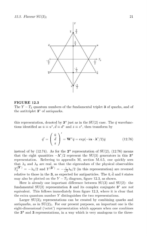
FIGURE 12.3
The Y − T 3 quantum numbers of the fundamental triplet 3 of quarks, and of
the antitriplet 3
∗ of antiquarks.
this representation, denoted by 3* just as in the SU(2) case. The q ¯ wavefunc¯
tions identified as u ¯ ≡ u
∗ , d ≡ d
∗ and s ¯ ≡ s
∗ , then transform by
(
)
u ¯
′
¯
q ¯
′ = ( d ) = W
∗ q ¯ = exp(−iα · λ
∗ /2)q ¯
(12.76)
s ¯
instead of by (12.74). As for the 2* representation of SU(2), (12.76) means
that the eight quantities −λ
∗ /2 represent the SU(3) generators in this 3*
representation. Referring to appendix M, section M.4.5, one quickly sees
that λ 3 and λ 8 are real, so that the eigenvalues of the physical observables
(3
∗ )
∗
T 3
−
3
= λ 3 /2 and Y
( ) = − √ 1 λ 8 /2 (in this representation) are reversed
3
¯
relative to those in the 3, as expected for antiparticles. The u ¯, d and ¯ s states
may also be plotted on the Y − T 3 diagram, figure 12.3, as shown.
Here is already one important difference between SU(3) and SU(2): the
fundamental SU(3) representation 3 and its complex conjugate 3
∗ are not
equivalent. This follows immediately from figure 12.3, where it is clear that
the extra quantum number Y distinguishes the two representations.
Larger SU(3) f representations can be created by combining quarks and
antiquarks, as in SU(2) f . For our present purposes, an important one is the
eight-dimensional (‘octet’) representation which appears when one combines
the 3* and 3 representations, in a way which is very analogous to the three-
21
FIGURE 12.3
The Y − T 3 quantum numbers of the fundamental triplet 3 of quarks, and of
the antitriplet 3
∗ of antiquarks.
this representation, denoted by 3* just as in the SU(2) case. The q ¯ wavefunc¯
tions identified as u ¯ ≡ u
∗ , d ≡ d
∗ and s ¯ ≡ s
∗ , then transform by
(
)
u ¯
′
¯
q ¯
′ = ( d ) = W
∗ q ¯ = exp(−iα · λ
∗ /2)q ¯
(12.76)
s ¯
instead of by (12.74). As for the 2* representation of SU(2), (12.76) means
that the eight quantities −λ
∗ /2 represent the SU(3) generators in this 3*
representation. Referring to appendix M, section M.4.5, one quickly sees
that λ 3 and λ 8 are real, so that the eigenvalues of the physical observables
(3
∗ )
∗
T 3
−
3
= λ 3 /2 and Y
( ) = − √ 1 λ 8 /2 (in this representation) are reversed
3
¯
relative to those in the 3, as expected for antiparticles. The u ¯, d and ¯ s states
may also be plotted on the Y − T 3 diagram, figure 12.3, as shown.
Here is already one important difference between SU(3) and SU(2): the
fundamental SU(3) representation 3 and its complex conjugate 3
∗ are not
equivalent. This follows immediately from figure 12.3, where it is clear that
the extra quantum number Y distinguishes the two representations.
Larger SU(3) f representations can be created by combining quarks and
antiquarks, as in SU(2) f . For our present purposes, an important one is the
eight-dimensional (‘octet’) representation which appears when one combines
the 3* and 3 representations, in a way which is very analogous to the three-