

11
12.2. The flavour symmetry SU(2) f
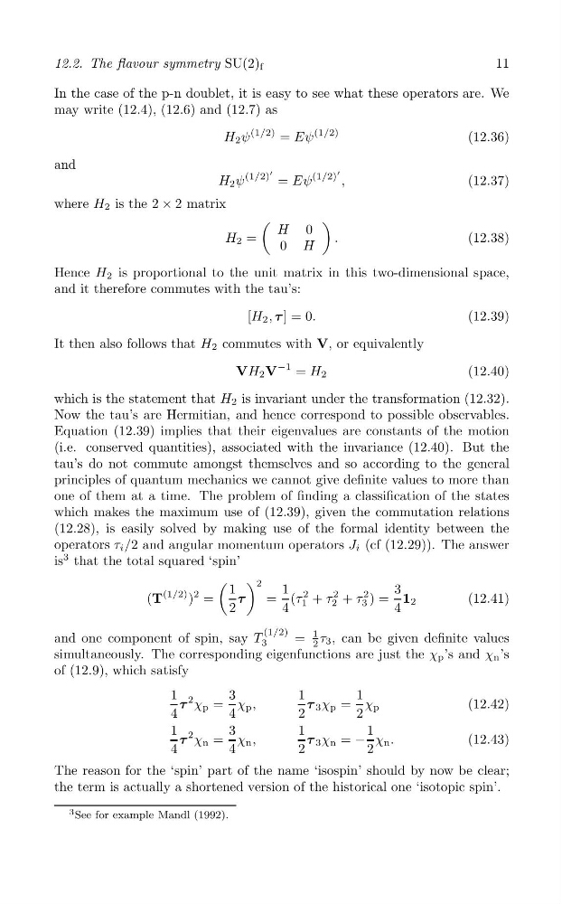
In the case of the p-n doublet, it is easy to see what these operators are. We
may write (12.4), (12.6) and (12.7) as
H 2 ψ
(1/2)
Eψ
(1/2)
=
(12.36)
and
H 2 ψ
(1/2)
′
Eψ
(1/2)
′
=
,
(12.37)
where H 2 is the 2 × 2 matrix
(
)
H 0
H 2 =
.
(12.38)
0 H
Hence H 2 is proportional to the unit matrix in this two-dimensional space,
and it therefore commutes with the tau’s:
[H 2 , τ ] = 0.
(12.39)
It then also follows that H 2 commutes with V, or equivalently
VH 2 V
−1 = H 2
(12.40)
which is the statement that H 2 is invariant under the transformation (12.32).
Now the tau’s are Hermitian, and hence correspond to possible observables.
Equation (12.39) implies that their eigenvalues are constants of the motion
(i.e. conserved quantities), associated with the invariance (12.40). But the
tau’s do not commute amongst themselves and so according to the general
principles of quantum mechanics we cannot give definite values to more than
one of them at a time. The problem of finding a classification of the states
which makes the maximum use of (12.39), given the commutation relations
(12.28), is easily solved by making use of the formal identity between the
operators τ i /2 and angular momentum operators J i (cf (12.29)). The answer
is
3 that the total squared ‘spin’
( ) 2
(T
(1/2) )
2
1
3
=
τ
=
1 (τ
2 + τ 2
2 + τ 3
2 ) = 1 2
(12.41)
1
2
4
4
(1/2)
1
and one component of spin, say T 3
= 2 τ 3 , can be given definite values
simultaneously. The corresponding eigenfunctions are just the χ p ’s and χ n ’s
of (12.9), which satisfy
1
3
1
1
τ
2 χ p = χ p ,
τ 3 χ p = χ p
(12.42)
4
4
2
2
1
3
1
1
τ
2 χ n = χ n ,
τ 3 χ n = − χ n .
(12.43)
4
4
2
2
The reason for the ‘spin’ part of the name ‘isospin’ should by now be clear;
the term is actually a shortened version of the historical one ‘isotopic spin’.
3 See for example Mandl (1992).
12.2. The flavour symmetry SU(2) f
In the case of the p-n doublet, it is easy to see what these operators are. We
may write (12.4), (12.6) and (12.7) as
H 2 ψ
(1/2)
Eψ
(1/2)
=
(12.36)
and
H 2 ψ
(1/2)
′
Eψ
(1/2)
′
=
,
(12.37)
where H 2 is the 2 × 2 matrix
(
)
H 0
H 2 =
.
(12.38)
0 H
Hence H 2 is proportional to the unit matrix in this two-dimensional space,
and it therefore commutes with the tau’s:
[H 2 , τ ] = 0.
(12.39)
It then also follows that H 2 commutes with V, or equivalently
VH 2 V
−1 = H 2
(12.40)
which is the statement that H 2 is invariant under the transformation (12.32).
Now the tau’s are Hermitian, and hence correspond to possible observables.
Equation (12.39) implies that their eigenvalues are constants of the motion
(i.e. conserved quantities), associated with the invariance (12.40). But the
tau’s do not commute amongst themselves and so according to the general
principles of quantum mechanics we cannot give definite values to more than
one of them at a time. The problem of finding a classification of the states
which makes the maximum use of (12.39), given the commutation relations
(12.28), is easily solved by making use of the formal identity between the
operators τ i /2 and angular momentum operators J i (cf (12.29)). The answer
is
3 that the total squared ‘spin’
( ) 2
(T
(1/2) )
2
1
3
=
τ
=
1 (τ
2 + τ 2
2 + τ 3
2 ) = 1 2
(12.41)
1
2
4
4
(1/2)
1
and one component of spin, say T 3
= 2 τ 3 , can be given definite values
simultaneously. The corresponding eigenfunctions are just the χ p ’s and χ n ’s
of (12.9), which satisfy
1
3
1
1
τ
2 χ p = χ p ,
τ 3 χ p = χ p
(12.42)
4
4
2
2
1
3
1
1
τ
2 χ n = χ n ,
τ 3 χ n = − χ n .
(12.43)
4
4
2
2
The reason for the ‘spin’ part of the name ‘isospin’ should by now be clear;
the term is actually a shortened version of the historical one ‘isotopic spin’.
3 See for example Mandl (1992).