

403
H.3. Time-dependent approach
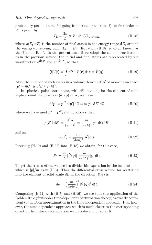
probability per unit time for going from state |i> to state |f>, to first order in
V , is given by
2π
˙
P fi =
||
2 ρ(E f )| E f =Ei
(H.18)
ħ
where ρ(E f )dE f is the number of final states in the energy range dE f around
the energy-conserving point E i = E f . Equation (H.18) is often known as
the ‘Golden Rule’. In the present case, if we adopt the same normalization
as in the previous section, the initial and final states are represented by the
wavefunction e
ik·r and e
−ik
' ·r , so that
∫
= e
iq·r V (r) d
3
r ≡ V ˜ (q).
(H.19)
′
Also, the number of such states in a volume element d
3
p of momentum space
′
(p = ħk
′ ) is d
3
p
′ /(2πħ)
3 .
In spherical polar coordinates, with dΩ standing for the element of solid
angle around the direction (θ, /φ) of p
′ , we have
′
′ 2
d
3
p = p d|p
′
| dΩ = m|p
′
| dE
′ dΩ
(H.20)
′ 2
where we have used E
′ = p /2m. It follows that
′
d
3
p
m
ρ(E
′ ) dE
′ =
=
|p
′
| dΩ dE
′
(H.21)
(2πħ) 3
(2πħ) 3
and so
m
ρ(E
′ ) =
|p
′
| dΩ.
(H.22)
(2πħ) 3
Inserting (H.19) and (H.22) into (H.18) we obtain, for this case,
2π
m
P ˙ fi =
|V ˜ (q)|
2
|p| dΩ.
(H.23)
ħ
(2πħ) 3
To get the cross section, we need to divide this expression by the incident flux,
which is |p|/m as in (H.3). Thus the differential cross section for scattering
into the element of solid angle dΩ in the direction (θ, φ) is
(
) 2
m
dσ =
|V ˜ (q)|
2 dΩ.
(H.24)
2πħ 2
Comparing (H.24) with (H.7) and (H.16), we see that this application of the
Golden Rule (first-order time-dependent perturbation theory) is exactly equivalent to the Born approximation in the time-independent approach. It is, however, the time-dependent approach which is much closer to the corresponding
quantum field theory formulation we introduce in chapter 6.
H.3. Time-dependent approach
probability per unit time for going from state |i> to state |f>, to first order in
V , is given by
2π
˙
P fi =
|
2 ρ(E f )| E f =Ei
(H.18)
ħ
where ρ(E f )dE f is the number of final states in the energy range dE f around
the energy-conserving point E i = E f . Equation (H.18) is often known as
the ‘Golden Rule’. In the present case, if we adopt the same normalization
as in the previous section, the initial and final states are represented by the
wavefunction e
ik·r and e
−ik
' ·r , so that
∫
iq·r V (r) d
3
r ≡ V ˜ (q).
(H.19)
′
Also, the number of such states in a volume element d
3
p of momentum space
′
(p = ħk
′ ) is d
3
p
′ /(2πħ)
3 .
In spherical polar coordinates, with dΩ standing for the element of solid
angle around the direction (θ, /φ) of p
′ , we have
′
′ 2
d
3
p = p d|p
′
| dΩ = m|p
′
| dE
′ dΩ
(H.20)
′ 2
where we have used E
′ = p /2m. It follows that
′
d
3
p
m
ρ(E
′ ) dE
′ =
=
|p
′
| dΩ dE
′
(H.21)
(2πħ) 3
(2πħ) 3
and so
m
ρ(E
′ ) =
|p
′
| dΩ.
(H.22)
(2πħ) 3
Inserting (H.19) and (H.22) into (H.18) we obtain, for this case,
2π
m
P ˙ fi =
|V ˜ (q)|
2
|p| dΩ.
(H.23)
ħ
(2πħ) 3
To get the cross section, we need to divide this expression by the incident flux,
which is |p|/m as in (H.3). Thus the differential cross section for scattering
into the element of solid angle dΩ in the direction (θ, φ) is
(
) 2
m
dσ =
|V ˜ (q)|
2 dΩ.
(H.24)
2πħ 2
Comparing (H.24) with (H.7) and (H.16), we see that this application of the
Golden Rule (first-order time-dependent perturbation theory) is exactly equivalent to the Born approximation in the time-independent approach. It is, however, the time-dependent approach which is much closer to the corresponding
quantum field theory formulation we introduce in chapter 6.