

397
G. Green Functions
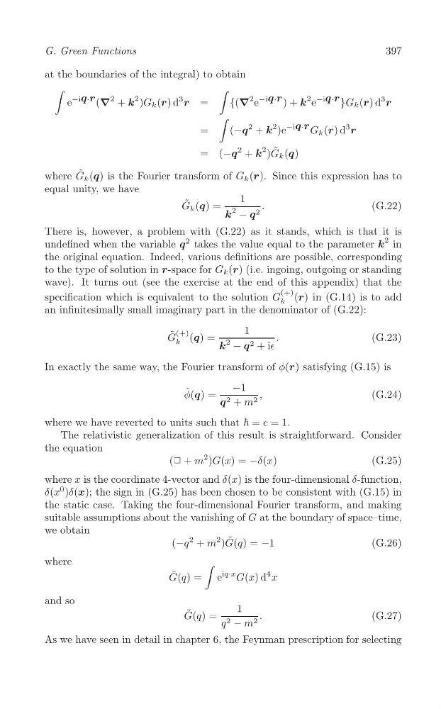
at the boundaries of the integral) to obtain
∫
∫
e
−iq·r (∇
2 + k
2 )G k (r) d
3
r =
{(∇
2 e
−iq·r ) + k
2 e
−iq·r
}G k (r) d
3
r
∫
2
=
(−q + k
2 )e
−iq·r G k (r) d
3
r
2
= (−q + k
2 )G ˜ k (q)
where G ˜ k (q) is the Fourier transform of G k (r). Since this expression has to
equal unity, we have
1
˜
G k (q) =
.
(G.22)
k
2
− q 2
There is, however, a problem with (G.22) as it stands, which is that it is
2
undefined when the variable q takes the value equal to the parameter k
2 in
the original equation. Indeed, various definitions are possible, corresponding
to the type of solution in r-space for G k (r) (i.e. ingoing, outgoing or standing
wave). It turns out (see the exercise at the end of this appendix) that the
(+)
specification which is equivalent to the solution G (r) in (G.14) is to add
k
an infinitesimally small imaginary part in the denominator of (G.22):
1
(+)
˜
G (q) =
.
(G.23)
k
k
2
− q 2 + i∈
In exactly the same way, the Fourier transform of φ(r) satisfying (G.15) is
−1
˜
φ(q) =
,
(G.24)
q 2 + m 2
where we have reverted to units such that ħ = c = 1.
The relativistic generalization of this result is straightforward. Consider
the equation
(❗ + m
2 )G(x) = −δ(x)
(G.25)
where x is the coordinate 4-vector and δ(x) is the four-dimensional δ-function,
δ(x
0 )δ(x); the sign in (G.25) has been chosen to be consistent with (G.15) in
the static case. Taking the four-dimensional Fourier transform, and making
suitable assumptions about the vanishing of G at the boundary of space–time,
we obtain
(−q
2 + m
2 ) ˜
G(q) = −1
(G.26)
where
∫
˜
G(q) = e
iq·x G(x) d
4 x
and so
1
˜
G(q) =
.
(G.27)
q 2 − m 2
As we have seen in detail in chapter 6, the Feynman prescription for selecting
G. Green Functions
at the boundaries of the integral) to obtain
∫
∫
e
−iq·r (∇
2 + k
2 )G k (r) d
3
r =
{(∇
2 e
−iq·r ) + k
2 e
−iq·r
}G k (r) d
3
r
∫
2
=
(−q + k
2 )e
−iq·r G k (r) d
3
r
2
= (−q + k
2 )G ˜ k (q)
where G ˜ k (q) is the Fourier transform of G k (r). Since this expression has to
equal unity, we have
1
˜
G k (q) =
.
(G.22)
k
2
− q 2
There is, however, a problem with (G.22) as it stands, which is that it is
2
undefined when the variable q takes the value equal to the parameter k
2 in
the original equation. Indeed, various definitions are possible, corresponding
to the type of solution in r-space for G k (r) (i.e. ingoing, outgoing or standing
wave). It turns out (see the exercise at the end of this appendix) that the
(+)
specification which is equivalent to the solution G (r) in (G.14) is to add
k
an infinitesimally small imaginary part in the denominator of (G.22):
1
(+)
˜
G (q) =
.
(G.23)
k
k
2
− q 2 + i∈
In exactly the same way, the Fourier transform of φ(r) satisfying (G.15) is
−1
˜
φ(q) =
,
(G.24)
q 2 + m 2
where we have reverted to units such that ħ = c = 1.
The relativistic generalization of this result is straightforward. Consider
the equation
(❗ + m
2 )G(x) = −δ(x)
(G.25)
where x is the coordinate 4-vector and δ(x) is the four-dimensional δ-function,
δ(x
0 )δ(x); the sign in (G.25) has been chosen to be consistent with (G.15) in
the static case. Taking the four-dimensional Fourier transform, and making
suitable assumptions about the vanishing of G at the boundary of space–time,
we obtain
(−q
2 + m
2 ) ˜
G(q) = −1
(G.26)
where
∫
˜
G(q) = e
iq·x G(x) d
4 x
and so
1
˜
G(q) =
.
(G.27)
q 2 − m 2
As we have seen in detail in chapter 6, the Feynman prescription for selecting