

381
E. Dirac δ-Function
and similarly from (E.14)
∫ ∞
g(k) =
f (x)e
−ikx dx.
(E.21)
−∞
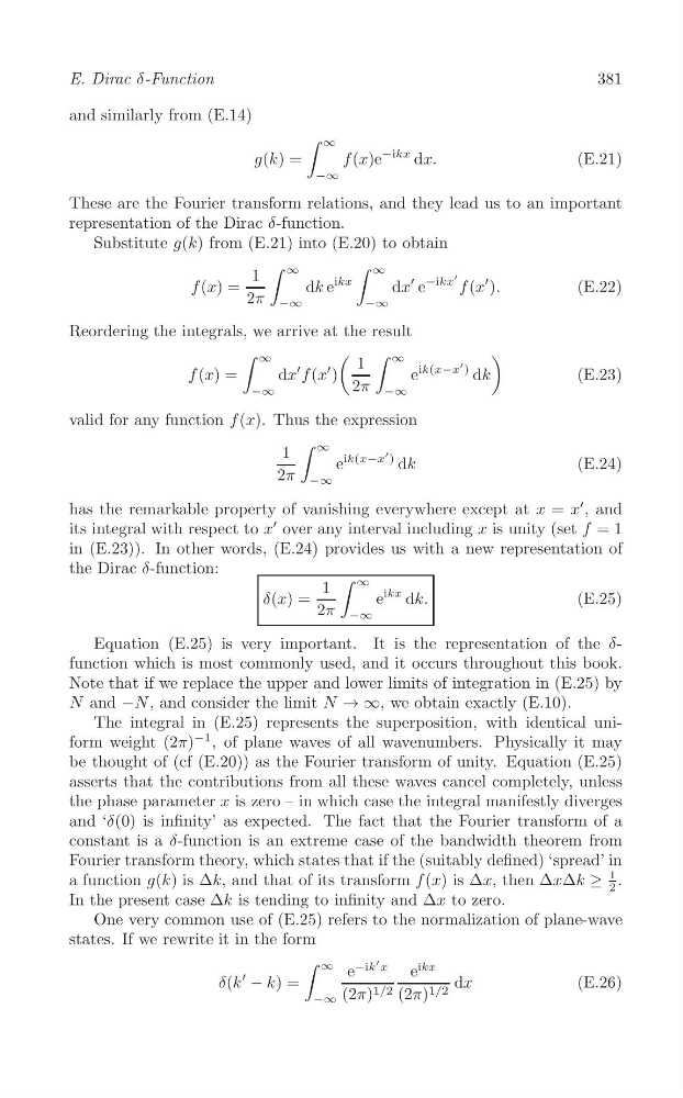
These are the Fourier transform relations, and they lead us to an important
representation of the Dirac δ-function.
Substitute g(k) from (E.21) into (E.20) to obtain
∫
∫
∞
∞
1
ikx
′ −ikx
'
′ ).
f (x) =
dk e
dx e
f (x
(E.22)
2π −∞
−∞
Reordering the integrals, we arrive at the result
(
)
∫
∫
∞
∞
ik(x−x
f (x) =
dx
′ f (x
′ )
1
e
' ) dk
(E.23)
2π
−∞
−∞
valid for any function f (x). Thus the expression
∫ ∞
ik(x−x
1
e
' ) dk
(E.24)
2π −∞
has the remarkable property of vanishing everywhere except at x = x
′ , and
′
its integral with respect to x over any interval including x is unity (set f = 1
in (E.23)). In other words, (E.24) provides us with a new representation of
the Dirac δ-function:
∫ ∞
δ(x) =
1
e
ikx dk.
(E.25)
2π −∞
Equation (E.25) is very important. It is the representation of the δfunction which is most commonly used, and it occurs throughout this book.
Note that if we replace the upper and lower limits of integration in (E.25) by
N and −N , and consider the limit N → ∞, we obtain exactly (E.10).
The integral in (E.25) represents the superposition, with identical uniform weight (2π)
−1 , of plane waves of all wavenumbers. Physically it may
be thought of (cf (E.20)) as the Fourier transform of unity. Equation (E.25)
asserts that the contributions from all these waves cancel completely, unless
the phase parameter x is zero – in which case the integral manifestly diverges
and ‘δ(0) is infinity’ as expected. The fact that the Fourier transform of a
constant is a δ-function is an extreme case of the bandwidth theorem from
Fourier transform theory, which states that if the (suitably defined) ‘spread’ in
a function g(k) is Δk, and that of its transform f (x) is Δx, then ΔxΔk ≥
1 .
In the present case Δk is tending to infinity and Δx to zero.
One very common use of (E.25) refers to the normalization of plane-wave
states. If we rewrite it in the form
∫ ∞ −ik
' x
ikx
e
e
δ(k
′
− k) =
dx
(E.26)
−∞ (2π) 1/2 (2π) 1/2
2
E. Dirac δ-Function
and similarly from (E.14)
∫ ∞
g(k) =
f (x)e
−ikx dx.
(E.21)
−∞
These are the Fourier transform relations, and they lead us to an important
representation of the Dirac δ-function.
Substitute g(k) from (E.21) into (E.20) to obtain
∫
∫
∞
∞
1
ikx
′ −ikx
'
′ ).
f (x) =
dk e
dx e
f (x
(E.22)
2π −∞
−∞
Reordering the integrals, we arrive at the result
(
)
∫
∫
∞
∞
ik(x−x
f (x) =
dx
′ f (x
′ )
1
e
' ) dk
(E.23)
2π
−∞
−∞
valid for any function f (x). Thus the expression
∫ ∞
ik(x−x
1
e
' ) dk
(E.24)
2π −∞
has the remarkable property of vanishing everywhere except at x = x
′ , and
′
its integral with respect to x over any interval including x is unity (set f = 1
in (E.23)). In other words, (E.24) provides us with a new representation of
the Dirac δ-function:
∫ ∞
δ(x) =
1
e
ikx dk.
(E.25)
2π −∞
Equation (E.25) is very important. It is the representation of the δfunction which is most commonly used, and it occurs throughout this book.
Note that if we replace the upper and lower limits of integration in (E.25) by
N and −N , and consider the limit N → ∞, we obtain exactly (E.10).
The integral in (E.25) represents the superposition, with identical uniform weight (2π)
−1 , of plane waves of all wavenumbers. Physically it may
be thought of (cf (E.20)) as the Fourier transform of unity. Equation (E.25)
asserts that the contributions from all these waves cancel completely, unless
the phase parameter x is zero – in which case the integral manifestly diverges
and ‘δ(0) is infinity’ as expected. The fact that the Fourier transform of a
constant is a δ-function is an extreme case of the bandwidth theorem from
Fourier transform theory, which states that if the (suitably defined) ‘spread’ in
a function g(k) is Δk, and that of its transform f (x) is Δx, then ΔxΔk ≥
1 .
In the present case Δk is tending to infinity and Δx to zero.
One very common use of (E.25) refers to the normalization of plane-wave
states. If we rewrite it in the form
∫ ∞ −ik
' x
ikx
e
e
δ(k
′
− k) =
dx
(E.26)
−∞ (2π) 1/2 (2π) 1/2
2