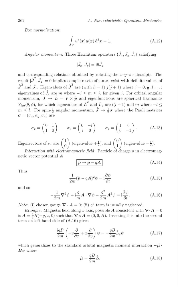
362
A. Non-relativistic Quantum Mechanics
Box normalization:
∫
u
∗ (x)u(x) d
3
x = 1.
(A.12)
V
ˆ ˆ
Angular momentum: Three Hermitian operators ( J ˆ x , J y , J z ) satisfying

[J ˆ x , J ˆ y ] = iħJ ˆ z
and corresponding relations obtained by rotating the x–y–z subscripts. The

2
result [J ˆ , ˆ
J z ] = 0 implies complete sets of states exist with definite values of
2
2
ˆ
J and J ˆ z . Eigenvalues of J ˆ are (with ħ = 1) j(j + 1) where j = 0,
1
2 , 1, . . . ;
eigenvalues of J ˆ z are m where −j ≤ m ≤ j, for given j. For orbital angular
momentum, J ˆ → L ˆ = r × p ˆ and eigenfunctions are spherical harmonics
2
(θ, φ), for which eigenvalues of L ˆ and L ˆ z are l(l + 1) and m where −l ≤
Y em
For spin1
2 angular momentum, J ˆ →
1
2 σ where the Pauli matrices
m ≤ l.
σ = (σ x , σ y , σ z ) are
σ x =
(
0 1
1 0
)
σ y =
(
0
i
−i
0
)
σ z =
(
1
0
0
−1
)
.
(A.13)
Eigenvectors of s z are
( )
1
0
Interaction with electromagnetic field : Particle of charge q in electromag(eigenvalue +
1
2 ), and
( )
0
1
(eigenvalue −
1
2 ).
netic vector potential A
ˆ
p → ˆ
p − qA .
(A.14)
Thus
and so
1
2m
(ˆ p − qA)
2 ψ = i
∂ψ
∂t
(A.15)
2
q
2m
m
2m
∂t
Note: (i) chosen gauge ∇ · A = 0; (ii) q
2 term is usually neglected.
1
∂ψ
∇
2
q
ψ + i A · ∇ψ +
A
2
−
ψ = i
.
(A.16)
Example: Magnetic field along z-axis, possible A consistent with ∇·A = 0
is A =
1
2 B(−y, x, 0) such that ∇×A = (0, 0, B). Inserting this into the second
term on left-hand side of (A.16) gives
(
)
iqB
∂
∂
qB ˆ
−y
+ x
ψ = −
L z ψ
(A.17)
2m
∂x
∂y
2m
which generalizes to the standard orbital magnetic moment interaction −μ ˆ ·
Bψ where
qB ˆ
μ ˆ =
L.
(A.18)
2m