

[2]
11.5. The physics of Π ¯ γ (q
2 )
341
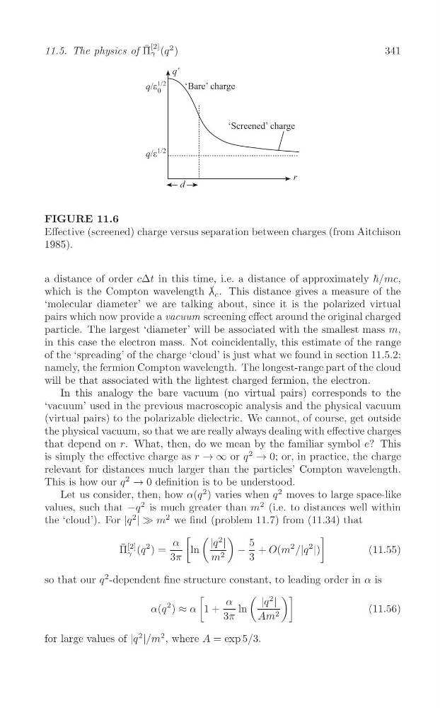
FIGURE 11.6
Effective (screened) charge versus separation between charges (from Aitchison
1985).
a distance of order cΔt in this time, i.e. a distance of approximately ħ/mc,
which is the Compton wavelength λ / c . This distance gives a measure of the
‘molecular diameter’ we are talking about, since it is the polarized virtual
pairs which now provide a vacuum screening effect around the original charged
particle. The largest ‘diameter’ will be associated with the smallest mass m,
in this case the electron mass. Not coincidentally, this estimate of the range
of the ‘spreading’ of the charge ‘cloud’ is just what we found in section 11.5.2:
namely, the fermion Compton wavelength. The longest-range part of the cloud
will be that associated with the lightest charged fermion, the electron.
In this analogy the bare vacuum (no virtual pairs) corresponds to the
‘vacuum’ used in the previous macroscopic analysis and the physical vacuum
(virtual pairs) to the polarizable dielectric. We cannot, of course, get outside
the physical vacuum, so that we are really always dealing with effective charges
that depend on r. What, then, do we mean by the familiar symbol e? This
is simply the effective charge as r → ∞ or q
2
→ 0; or, in practice, the charge
relevant for distances much larger than the particles’ Compton wavelength.
This is how our q
2
→ 0 definition is to be understood.
Let us consider, then, how α(q
2 ) varies when q
2 moves to large space-like
2
2
values, such that −q is much greater than m (i.e. to distances well within
the ‘cloud’). For |q
2
| ≫ m
2 we find (problem 11.7) from (11.34) that
[ (
)
]
α
|q
2
|
5
Π
[2]
¯ (q
2 ) =
2 /|q
2
|)
ln
− + O(m
(11.55)
γ
3π
m 2
3
so that our q
2 -dependent fine structure constant, to leading order in α is
[
(
)]
α
|q
2
|
α(q
2 ) ≈ α 1 +
ln
(11.56)
3π
Am 2
for large values of |q
2
|/m
2 , where A = exp 5/3.
11.5. The physics of Π ¯ γ (q
2 )
341
FIGURE 11.6
Effective (screened) charge versus separation between charges (from Aitchison
1985).
a distance of order cΔt in this time, i.e. a distance of approximately ħ/mc,
which is the Compton wavelength λ / c . This distance gives a measure of the
‘molecular diameter’ we are talking about, since it is the polarized virtual
pairs which now provide a vacuum screening effect around the original charged
particle. The largest ‘diameter’ will be associated with the smallest mass m,
in this case the electron mass. Not coincidentally, this estimate of the range
of the ‘spreading’ of the charge ‘cloud’ is just what we found in section 11.5.2:
namely, the fermion Compton wavelength. The longest-range part of the cloud
will be that associated with the lightest charged fermion, the electron.
In this analogy the bare vacuum (no virtual pairs) corresponds to the
‘vacuum’ used in the previous macroscopic analysis and the physical vacuum
(virtual pairs) to the polarizable dielectric. We cannot, of course, get outside
the physical vacuum, so that we are really always dealing with effective charges
that depend on r. What, then, do we mean by the familiar symbol e? This
is simply the effective charge as r → ∞ or q
2
→ 0; or, in practice, the charge
relevant for distances much larger than the particles’ Compton wavelength.
This is how our q
2
→ 0 definition is to be understood.
Let us consider, then, how α(q
2 ) varies when q
2 moves to large space-like
2
2
values, such that −q is much greater than m (i.e. to distances well within
the ‘cloud’). For |q
2
| ≫ m
2 we find (problem 11.7) from (11.34) that
[ (
)
]
α
|q
2
|
5
Π
[2]
¯ (q
2 ) =
2 /|q
2
|)
ln
− + O(m
(11.55)
γ
3π
m 2
3
so that our q
2 -dependent fine structure constant, to leading order in α is
[
(
)]
α
|q
2
|
α(q
2 ) ≈ α 1 +
ln
(11.56)
3π
Am 2
for large values of |q
2
|/m
2 , where A = exp 5/3.