

¯ [2] 2 )
11.5. The physics of Π γ (q
337
Yukawa potential
2 −r/a
−g e
N
4π
r
−1
where a = m (in units ħ = c = 1). As m U → 0 we arrive at the Coulomb
U
2
potential, associated with the propagator ∼1/q in the static (q 0 = 0) limit.
It follows that the corrected propagator (11.32) must represent a correction
to the 1/r Coulomb potential.
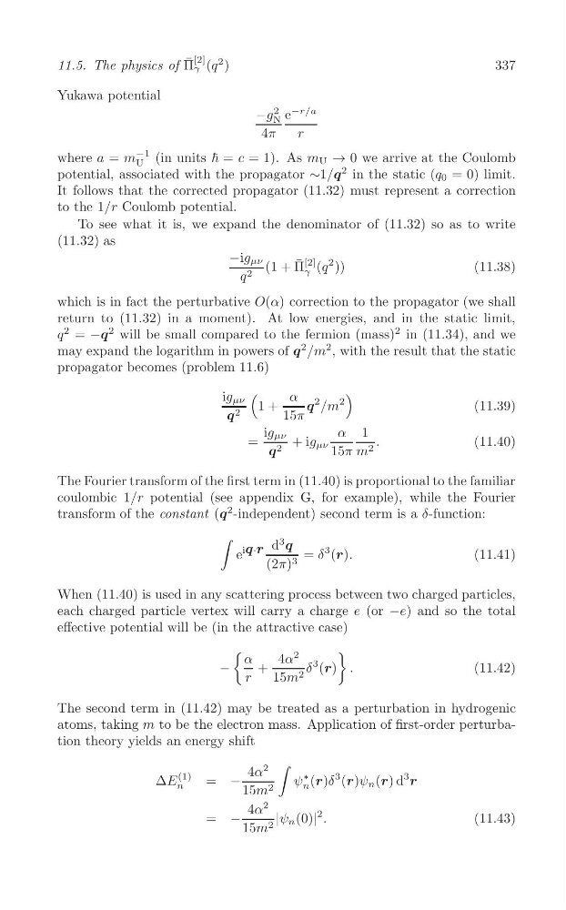
To see what it is, we expand the denominator of (11.32) so as to write
(11.32) as
−ig μν
Π
[2]
(1 + ¯ (q
2 ))
(11.38)
γ
q 2
which is in fact the perturbative O(α) correction to the propagator (we shall
return to (11.32) in a moment). At low energies, and in the static limit,
2
2
q = −q will be small compared to the fermion (mass)
2 in (11.34), and we
may expand the logarithm in powers of q
2 /m
2 , with the result that the static
propagator becomes (problem 11.6)
(
)
ig μν
α
1 +
q
2 /m
2
(11.39)
q 2
15π
ig μν
α 1
=
+ ig μν
.
(11.40)
q 2
15π m 2
The Fourier transform of the first term in (11.40) is proportional to the familiar
coulombic 1/r potential (see appendix G, for example), while the Fourier
transform of the constant (q
2 -independent) second term is a δ-function:
∫
d
3
q
e
iq·r
= δ
3 (r).
(11.41)
(2π) 3
When (11.40) is used in any scattering process between two charged particles,
each charged particle vertex will carry a charge e (or −e) and so the total
effective potential will be (in the attractive case)
(
)
α
4α
2
−
+
δ
3 (r) .
(11.42)
r
15m 2
The second term in (11.42) may be treated as a perturbation in hydrogenic
atoms, taking m to be the electron mass. Application of first-order perturbation theory yields an energy shift
∫
4α
2
ΔE
(1) = −
ψ
∗ (r)δ
3 (r)ψ n (r) d
3
r
n
n
15m 2
4α
2
= −
|ψ n (0)|
2 .
(11.43)
15m 2
11.5. The physics of Π γ (q
337
Yukawa potential
2 −r/a
−g e
N
4π
r
−1
where a = m (in units ħ = c = 1). As m U → 0 we arrive at the Coulomb
U
2
potential, associated with the propagator ∼1/q in the static (q 0 = 0) limit.
It follows that the corrected propagator (11.32) must represent a correction
to the 1/r Coulomb potential.
To see what it is, we expand the denominator of (11.32) so as to write
(11.32) as
−ig μν
Π
[2]
(1 + ¯ (q
2 ))
(11.38)
γ
q 2
which is in fact the perturbative O(α) correction to the propagator (we shall
return to (11.32) in a moment). At low energies, and in the static limit,
2
2
q = −q will be small compared to the fermion (mass)
2 in (11.34), and we
may expand the logarithm in powers of q
2 /m
2 , with the result that the static
propagator becomes (problem 11.6)
(
)
ig μν
α
1 +
q
2 /m
2
(11.39)
q 2
15π
ig μν
α 1
=
+ ig μν
.
(11.40)
q 2
15π m 2
The Fourier transform of the first term in (11.40) is proportional to the familiar
coulombic 1/r potential (see appendix G, for example), while the Fourier
transform of the constant (q
2 -independent) second term is a δ-function:
∫
d
3
q
e
iq·r
= δ
3 (r).
(11.41)
(2π) 3
When (11.40) is used in any scattering process between two charged particles,
each charged particle vertex will carry a charge e (or −e) and so the total
effective potential will be (in the attractive case)
(
)
α
4α
2
−
+
δ
3 (r) .
(11.42)
r
15m 2
The second term in (11.42) may be treated as a perturbation in hydrogenic
atoms, taking m to be the electron mass. Application of first-order perturbation theory yields an energy shift
∫
4α
2
ΔE
(1) = −
ψ
∗ (r)δ
3 (r)ψ n (r) d
3
r
n
n
15m 2
4α
2
= −
|ψ n (0)|
2 .
(11.43)
15m 2