

288
9. Deep Inelastic Electron–Nucleon Scattering and the Parton Model
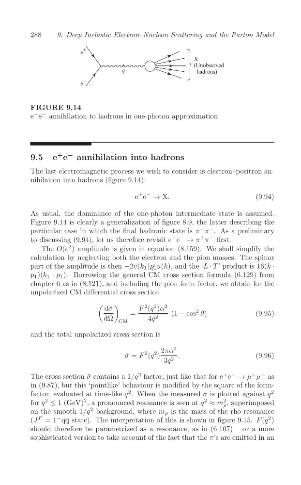
FIGURE 9.14
+
e e
− annihilation to hadrons in one-photon approximation.
+ −
9.5 e e annihilation into hadrons
The last electromagnetic process we wish to consider is electron–positron annihilation into hadrons (figure 9.14):
+
e e
−
→ X.
(9.94)
As usual, the dominance of the one-photon intermediate state is assumed.
Figure 9.14 is clearly a generalization of figure 8.9, the latter describing the
particular case in which the final hadronic state is π
+ π
− . As a preliminary
to discussing (9.94), let us therefore revisit e
+ e
−
→ π
+ π
− first.
The O(e
2 ) amplitude is given in equation (8.159). We shall simplify the
calculation by neglecting both the electron and the pion masses. The spinor
part of the amplitude is then −2¯ v(k 1 )p /1 u(k), and the ‘L · T ’ product is 16(k ·
p 1 )(k 1 · p 1 ). Borrowing the general CM cross section formula (6.129) from
chapter 6 as in (8.121), and including the pion form factor, we obtain for the
unpolarized CM differential cross section
(
)
d¯ σ
F
2 (q
2 )α
2
=
(1 − cos
2 θ)
(9.95)
dΩ
4q 2
CM
and the total unpolarized cross section is
2πα
2
σ ¯ = F
2 (q
2 )
.
(9.96)
3q 2
The cross section ¯
σ contains a 1/q
2 factor, just like that for e
+ e
−
→ μ
+ μ
− as
in (9.87), but this ‘pointlike’ behaviour is modified by the square of the form2
factor, evaluated at time-like q
2 . When the measured ¯
σ is plotted against q
2
for q
2
≤ 1 (GeV)
2 , a pronounced resonance is seen at q
2
≈ m ρ , superimposed
on the smooth 1/q
2 background, where m ρ is the mass of the rho resonance
(J
P = 1
− q¯ q state). The interpretation of this is shown in figure 9.15. F (q
2 )
should therefore be parametrized as a resonance, as in (6.107) – or a more
sophisticated version to take account of the fact that the π’s are emitted in an
9. Deep Inelastic Electron–Nucleon Scattering and the Parton Model
FIGURE 9.14
+
e e
− annihilation to hadrons in one-photon approximation.
+ −
9.5 e e annihilation into hadrons
The last electromagnetic process we wish to consider is electron–positron annihilation into hadrons (figure 9.14):
+
e e
−
→ X.
(9.94)
As usual, the dominance of the one-photon intermediate state is assumed.
Figure 9.14 is clearly a generalization of figure 8.9, the latter describing the
particular case in which the final hadronic state is π
+ π
− . As a preliminary
to discussing (9.94), let us therefore revisit e
+ e
−
→ π
+ π
− first.
The O(e
2 ) amplitude is given in equation (8.159). We shall simplify the
calculation by neglecting both the electron and the pion masses. The spinor
part of the amplitude is then −2¯ v(k 1 )p /1 u(k), and the ‘L · T ’ product is 16(k ·
p 1 )(k 1 · p 1 ). Borrowing the general CM cross section formula (6.129) from
chapter 6 as in (8.121), and including the pion form factor, we obtain for the
unpolarized CM differential cross section
(
)
d¯ σ
F
2 (q
2 )α
2
=
(1 − cos
2 θ)
(9.95)
dΩ
4q 2
CM
and the total unpolarized cross section is
2πα
2
σ ¯ = F
2 (q
2 )
.
(9.96)
3q 2
The cross section ¯
σ contains a 1/q
2 factor, just like that for e
+ e
−
→ μ
+ μ
− as
in (9.87), but this ‘pointlike’ behaviour is modified by the square of the form2
factor, evaluated at time-like q
2 . When the measured ¯
σ is plotted against q
2
for q
2
≤ 1 (GeV)
2 , a pronounced resonance is seen at q
2
≈ m ρ , superimposed
on the smooth 1/q
2 background, where m ρ is the mass of the rho resonance
(J
P = 1
− q¯ q state). The interpretation of this is shown in figure 9.15. F (q
2 )
should therefore be parametrized as a resonance, as in (6.107) – or a more
sophisticated version to take account of the fact that the π’s are emitted in an