

251
8.6. Electron Compton scattering
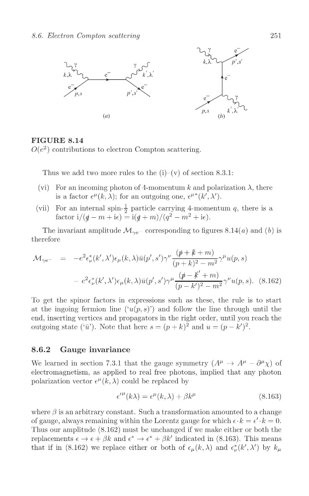
FIGURE 8.14
O(e
2 ) contributions to electron Compton scattering.
Thus we add two more rules to the (i)–(v) of section 8.3.1:
(vi) For an incoming photon of 4-momentum k and polarization λ, there
is a factor ∈
μ (k, λ); for an outgoing one, ∈
μ∗ (k
′ , λ
′ ).
(vii) For an internal spin1 particle carrying 4-momentum q, there is a
2
factor i/( / q − m + i∈) = i( / q + m)/(q
2
− m
2 + i∈).
The invariant amplitude M γe − corresponding to figures 8.14(a) and (b) is
therefore
( / p + k / + m)
′
M γe − = −e
2 ∈
∗
ν (k
′ , λ
′ )∈ μ (k, λ)¯ u(p , s
′ )γ
ν
γ
μ u(p, s)
(p + k) 2 − m 2
′
( / p − k / + m)
2 ∈
∗
′ ′ )γ
μ
γ
ν
− e ν (k
′ , λ
′ )∈ μ (k, λ)¯ u(p , s
u(p, s). (8.162)
(p − k ′ ) 2 − m 2
To get the spinor factors in expressions such as these, the rule is to start
at the ingoing fermion line (‘u(p, s)’) and follow the line through until the
end, inserting vertices and propagators in the right order, until you reach the
outgoing state (‘¯ u’). Note that here s = (p + k)
2 and u = (p − k
′ )
2 .
8.6.2 Gauge invariance
We learned in section 7.3.1 that the gauge symmetry (A
μ
→ A
μ
− ∂
μ χ) of
electromagnetism, as applied to real free photons, implied that any photon
polarization vector ∈
μ (k, λ) could be replaced by
∈
′ μ (kλ) = ∈
μ (k, λ) + βk
μ
(8.163)
where β is an arbitrary constant. Such a transformation amounted to a change
of gauge, always remaining within the Lorentz gauge for which ∈·k = ∈
′
·k = 0.
Thus our amplitude (8.162) must be unchanged if we make either or both the
replacements ∈ → ∈ + βk and ∈
∗
→ ∈
∗ + βk
′ indicated in (8.163). This means
that if in (8.162) we replace either or both of ∈ μ (k, λ) and ∈
∗
ν (k
′ , λ
′ ) by k μ
8.6. Electron Compton scattering
FIGURE 8.14
O(e
2 ) contributions to electron Compton scattering.
Thus we add two more rules to the (i)–(v) of section 8.3.1:
(vi) For an incoming photon of 4-momentum k and polarization λ, there
is a factor ∈
μ (k, λ); for an outgoing one, ∈
μ∗ (k
′ , λ
′ ).
(vii) For an internal spin1 particle carrying 4-momentum q, there is a
2
factor i/( / q − m + i∈) = i( / q + m)/(q
2
− m
2 + i∈).
The invariant amplitude M γe − corresponding to figures 8.14(a) and (b) is
therefore
( / p + k / + m)
′
M γe − = −e
2 ∈
∗
ν (k
′ , λ
′ )∈ μ (k, λ)¯ u(p , s
′ )γ
ν
γ
μ u(p, s)
(p + k) 2 − m 2
′
( / p − k / + m)
2 ∈
∗
′ ′ )γ
μ
γ
ν
− e ν (k
′ , λ
′ )∈ μ (k, λ)¯ u(p , s
u(p, s). (8.162)
(p − k ′ ) 2 − m 2
To get the spinor factors in expressions such as these, the rule is to start
at the ingoing fermion line (‘u(p, s)’) and follow the line through until the
end, inserting vertices and propagators in the right order, until you reach the
outgoing state (‘¯ u’). Note that here s = (p + k)
2 and u = (p − k
′ )
2 .
8.6.2 Gauge invariance
We learned in section 7.3.1 that the gauge symmetry (A
μ
→ A
μ
− ∂
μ χ) of
electromagnetism, as applied to real free photons, implied that any photon
polarization vector ∈
μ (k, λ) could be replaced by
∈
′ μ (kλ) = ∈
μ (k, λ) + βk
μ
(8.163)
where β is an arbitrary constant. Such a transformation amounted to a change
of gauge, always remaining within the Lorentz gauge for which ∈·k = ∈
′
·k = 0.
Thus our amplitude (8.162) must be unchanged if we make either or both the
replacements ∈ → ∈ + βk and ∈
∗
→ ∈
∗ + βk
′ indicated in (8.163). This means
that if in (8.162) we replace either or both of ∈ μ (k, λ) and ∈
∗
ν (k
′ , λ
′ ) by k μ