

243
8.4. Scattering from a non-point-like object
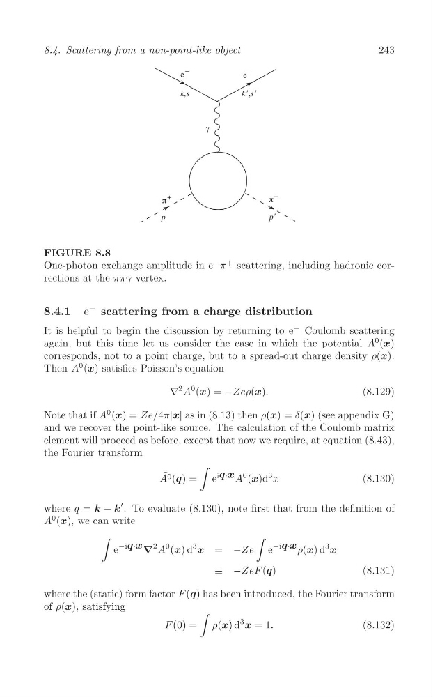
FIGURE 8.8
One-photon exchange amplitude in e
− π
+ scattering, including hadronic corrections at the ππγ vertex.
8.4.1 e − scattering from a charge distribution
It is helpful to begin the discussion by returning to e
− Coulomb scattering
again, but this time let us consider the case in which the potential A
0 (x)
corresponds, not to a point charge, but to a spread-out charge density ρ(x).
Then A
0 (x) satisfies Poisson’s equation
∇
2 A
0 (x) = −Zeρ(x).
(8.129)
Note that if A
0 (x) = Ze/4π|x| as in (8.13) then ρ(x) = δ(x) (see appendix G)
and we recover the point-like source. The calculation of the Coulomb matrix
element will proceed as before, except that now we require, at equation (8.43),
the Fourier transform
∫
A ˜0 (q) = e
iq·x A
0 (x)d
3 x
(8.130)
k
′
where q = k − . To evaluate (8.130), note first that from the definition of
A
0 (x), we can write
∫
∫
e
−iq·x
∇
2 A
0 (x) d
3
x = −Ze e
−iq·x ρ(x) d
3
x
≡ −ZeF (q)
(8.131)
where the (static) form factor F (q) has been introduced, the Fourier transform
of ρ(x), satisfying
∫
F (0) = ρ(x) d
3
x = 1.
(8.132)
8.4. Scattering from a non-point-like object
FIGURE 8.8
One-photon exchange amplitude in e
− π
+ scattering, including hadronic corrections at the ππγ vertex.
8.4.1 e − scattering from a charge distribution
It is helpful to begin the discussion by returning to e
− Coulomb scattering
again, but this time let us consider the case in which the potential A
0 (x)
corresponds, not to a point charge, but to a spread-out charge density ρ(x).
Then A
0 (x) satisfies Poisson’s equation
∇
2 A
0 (x) = −Zeρ(x).
(8.129)
Note that if A
0 (x) = Ze/4π|x| as in (8.13) then ρ(x) = δ(x) (see appendix G)
and we recover the point-like source. The calculation of the Coulomb matrix
element will proceed as before, except that now we require, at equation (8.43),
the Fourier transform
∫
A ˜0 (q) = e
iq·x A
0 (x)d
3 x
(8.130)
k
′
where q = k − . To evaluate (8.130), note first that from the definition of
A
0 (x), we can write
∫
∫
e
−iq·x
∇
2 A
0 (x) d
3
x = −Ze e
−iq·x ρ(x) d
3
x
≡ −ZeF (q)
(8.131)
where the (static) form factor F (q) has been introduced, the Fourier transform
of ρ(x), satisfying
∫
F (0) = ρ(x) d
3
x = 1.
(8.132)