

8.3. e
− s
+ scattering
235
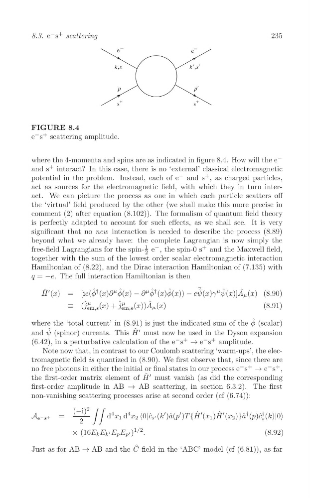
FIGURE 8.4
e
− s
+ scattering amplitude.
where the 4-momenta and spins are as indicated in figure 8.4. How will the e
−
and s
+ interact? In this case, there is no ‘external’ classical electromagnetic
potential in the problem. Instead, each of e
− and s
+ , as charged particles,
act as sources for the electromagnetic field, with which they in turn interact. We can picture the process as one in which each particle scatters off
the ‘virtual’ field produced by the other (we shall make this more precise in
comment (2) after equation (8.102)). The formalism of quantum field theory
is perfectly adapted to account for such effects, as we shall see. It is very
significant that no new interaction is needed to describe the process (8.89)
beyond what we already have: the complete Lagrangian is now simply the
free-field Lagrangians for the spin1 e
− , the spin-0 s
+ and the Maxwell field,
2
together with the sum of the lowest order scalar electromagnetic interaction
Hamiltonian of (8.22), and the Dirac interaction Hamiltonian of (7.135) with
q = −e. The full interaction Hamiltonian is then
H ˆ ′ (x) = [ie(φ ˆ † (x)∂
μ φ ˆ (x) − ∂
μ φ ˆ † (x)φ ˆ (x)) − eψ
¯ ˆ (x)γ
μ ψ ˆ (x)]A ˆ μ (x) (8.90)
( ˆ j
μ
j
μ
≡
em,s (x) + ˆ em,e (x))A ˆ μ (x)
(8.91)
where the ‘total current’ in (8.91) is just the indicated sum of the φ ˆ (scalar)
′
and ψ ˆ (spinor) currents. This H ˆ must now be used in the Dyson expansion
+
→
− +
(6.42), in a perturbative calculation of the e
− s
e s amplitude.
Note now that, in contrast to our Coulomb scattering ‘warm-ups’, the electromagnetic field is quantized in (8.90). We first observe that, since there are
−
− +
no free photons in either the initial or final states in our process e s
+
→ e s ,
′
the first-order matrix element of H ˆ must vanish (as did the corresponding
first-order amplitude in AB → AB scattering, in section 6.3.2). The first
non-vanishing scattering processes arise at second order (cf (6.74)):
∫ ∫
(−i)
2
†
A e − s + =
d
4 x 1 d
4 x 2 <0|c ˆ s ' (k
′ )ˆ a(p
′ )T {H ˆ ′ (x 1 )H ˆ ′ (x 2 )}a ˆ
† (p)ˆ c (k)|0>
s
2
× (16E k E k ' E p E p ' )
1/2 .
(8.92)
Just as for AB → AB and the C ˆ field in the ‘ABC’ model (cf (6.81)), as far
− s
+ scattering
235
FIGURE 8.4
e
− s
+ scattering amplitude.
where the 4-momenta and spins are as indicated in figure 8.4. How will the e
−
and s
+ interact? In this case, there is no ‘external’ classical electromagnetic
potential in the problem. Instead, each of e
− and s
+ , as charged particles,
act as sources for the electromagnetic field, with which they in turn interact. We can picture the process as one in which each particle scatters off
the ‘virtual’ field produced by the other (we shall make this more precise in
comment (2) after equation (8.102)). The formalism of quantum field theory
is perfectly adapted to account for such effects, as we shall see. It is very
significant that no new interaction is needed to describe the process (8.89)
beyond what we already have: the complete Lagrangian is now simply the
free-field Lagrangians for the spin1 e
− , the spin-0 s
+ and the Maxwell field,
2
together with the sum of the lowest order scalar electromagnetic interaction
Hamiltonian of (8.22), and the Dirac interaction Hamiltonian of (7.135) with
q = −e. The full interaction Hamiltonian is then
H ˆ ′ (x) = [ie(φ ˆ † (x)∂
μ φ ˆ (x) − ∂
μ φ ˆ † (x)φ ˆ (x)) − eψ
¯ ˆ (x)γ
μ ψ ˆ (x)]A ˆ μ (x) (8.90)
( ˆ j
μ
j
μ
≡
em,s (x) + ˆ em,e (x))A ˆ μ (x)
(8.91)
where the ‘total current’ in (8.91) is just the indicated sum of the φ ˆ (scalar)
′
and ψ ˆ (spinor) currents. This H ˆ must now be used in the Dyson expansion
+
→
− +
(6.42), in a perturbative calculation of the e
− s
e s amplitude.
Note now that, in contrast to our Coulomb scattering ‘warm-ups’, the electromagnetic field is quantized in (8.90). We first observe that, since there are
−
− +
no free photons in either the initial or final states in our process e s
+
→ e s ,
′
the first-order matrix element of H ˆ must vanish (as did the corresponding
first-order amplitude in AB → AB scattering, in section 6.3.2). The first
non-vanishing scattering processes arise at second order (cf (6.74)):
∫ ∫
(−i)
2
†
A e − s + =
d
4 x 1 d
4 x 2 <0|c ˆ s ' (k
′ )ˆ a(p
′ )T {H ˆ ′ (x 1 )H ˆ ′ (x 2 )}a ˆ
† (p)ˆ c (k)|0>
s
2
× (16E k E k ' E p E p ' )
1/2 .
(8.92)
Just as for AB → AB and the C ˆ field in the ‘ABC’ model (cf (6.81)), as far