

209
7.4. Introduction of electromagnetic interactions
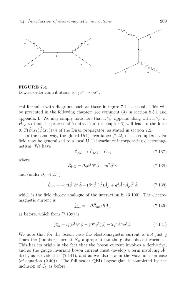
FIGURE 7.4
Lowest-order contributions to γe
−
→ γe
− .
ical formulae with diagrams such as those in figure 7.4, as usual. This will
be presented in the following chapter: see comment (3) in section 8.3.1 and
ˆ
¯ ˆ
appendix L. We may simply note here that a ‘ψ’ appears along with a ‘ψ’ in
ˆ ′
H , so that the process of ‘contraction’ (cf chapter 6) will lead to the form
D
¯ ˆ
<0|T (ψ ˆ (x 1 )ψ(x 2 ))|0> of the Dirac propagator, as stated in section 7.2.
In the same way, the global U(1) invariance (7.22) of the complex scalar
field may be generalized to a local U(1) invariance incorporating electromagnetism. We have
ˆ
L KG → ˆ
L KG + ˆ
L int
(7.137)
where
ˆ
L KG = ∂ μ ˆ
φ
† ∂
μ ˆ
φ − m
2 ˆ
φ
† ˆ
φ
(7.138)
and (under ∂ μ → ˆ
D μ )
L ˆ int = −iq(φ ˆ † ∂
μ φ ˆ − (∂
μ φ ˆ † )φ ˆ )A ˆ μ + q
2 A ˆ μ A ˆ μ φ ˆ † φ ˆ
(7.139)
which is the field theory analogue of the interaction in (3.100). The electromagnetic current is
ˆ j
μ = −∂L ˆ int /∂A ˆ μ
(7.140)
em
as before, which from (7.139) is
ˆ j
μ
φ
† ∂
μ φ ˆ − (∂
μ φ ˆ † ) ˆ
2 A ˆ μ φ ˆ † ˆ
= iq( ˆ
φ) − 2q
φ.
(7.141)
em
We note that for the boson case the electromagnetic current is not just q
times the (number) current N ˆ φ appropriate to the global phase invariance.
This has its origin in the fact that the boson current involves a derivative,
and so the gauge invariant boson current must develop a term involving A ˆ μ
itself, as is evident in (7.141), and as we also saw in the wavefunction case
(cf equation (2.40)). The full scalar QED Lagrangian is completed by the
inclusion of L ˆ ξ as before.
7.4. Introduction of electromagnetic interactions
FIGURE 7.4
Lowest-order contributions to γe
−
→ γe
− .
ical formulae with diagrams such as those in figure 7.4, as usual. This will
be presented in the following chapter: see comment (3) in section 8.3.1 and
ˆ
¯ ˆ
appendix L. We may simply note here that a ‘ψ’ appears along with a ‘ψ’ in
ˆ ′
H , so that the process of ‘contraction’ (cf chapter 6) will lead to the form
D
¯ ˆ
<0|T (ψ ˆ (x 1 )ψ(x 2 ))|0> of the Dirac propagator, as stated in section 7.2.
In the same way, the global U(1) invariance (7.22) of the complex scalar
field may be generalized to a local U(1) invariance incorporating electromagnetism. We have
ˆ
L KG → ˆ
L KG + ˆ
L int
(7.137)
where
ˆ
L KG = ∂ μ ˆ
φ
† ∂
μ ˆ
φ − m
2 ˆ
φ
† ˆ
φ
(7.138)
and (under ∂ μ → ˆ
D μ )
L ˆ int = −iq(φ ˆ † ∂
μ φ ˆ − (∂
μ φ ˆ † )φ ˆ )A ˆ μ + q
2 A ˆ μ A ˆ μ φ ˆ † φ ˆ
(7.139)
which is the field theory analogue of the interaction in (3.100). The electromagnetic current is
ˆ j
μ = −∂L ˆ int /∂A ˆ μ
(7.140)
em
as before, which from (7.139) is
ˆ j
μ
φ
† ∂
μ φ ˆ − (∂
μ φ ˆ † ) ˆ
2 A ˆ μ φ ˆ † ˆ
= iq( ˆ
φ) − 2q
φ.
(7.141)
em
We note that for the boson case the electromagnetic current is not just q
times the (number) current N ˆ φ appropriate to the global phase invariance.
This has its origin in the fact that the boson current involves a derivative,
and so the gauge invariant boson current must develop a term involving A ˆ μ
itself, as is evident in (7.141), and as we also saw in the wavefunction case
(cf equation (2.40)). The full scalar QED Lagrangian is completed by the
inclusion of L ˆ ξ as before.