

204
7. Quantum Field Theory III
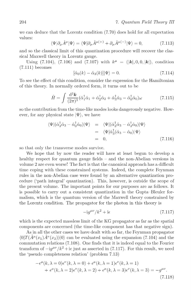
we can deduce that the Lorentz condition (7.70) does hold for all expectation
values:
ˆ
A ˆ μ(+)
ˆ
<Ψ|∂ μ A
μ
|Ψ> = <Ψ|∂ μ
+ ∂ μ A
μ(−)
|Ψ> = 0,
(7.113)
and so the classical limit of this quantization procedure will recover the classical Maxwell theory in Lorentz gauge.
Using (7.104), (7.106) and (7.107) with k
μ = (|k|, 0, 0, |k|), condition
(7.111) becomes
[ˆ α 0 (k) − α ˆ 3 (k)]|Ψ> = 0.
(7.114)
To see the effect of this condition, consider the expression for the Hamiltonian
of this theory. In normally ordered form, it turns out to be
∫ d
3
k
ˆ
H =
(2π) 3 (ˆ α
†
1 α ˆ 1 + ˆ
α
†
2 α ˆ 2 + ˆ
α
†
3 α ˆ 3 − α ˆ
†
0 α ˆ 0 )ω
(7.115)
so the contribution from the time-like modes looks dangerously negative. However, for any physical state |Ψ>, we have
<Ψ|(ˆ α
†
3 α ˆ 3 − α ˆ
†
0 α ˆ 0 )|Ψ>
†
3 α ˆ 3 − α ˆ
†
3 α ˆ 0 )|Ψ>
†
<Ψ|(ˆ α
=
<Ψ|α ˆ 3 (ˆ α 3 − α ˆ 0 )|Ψ>
=
= 0,
(7.116)
so that only the transverse modes survive.
We hope that by now the reader will have at least begun to develop a
healthy respect for quantum gauge fields – and the non-Abelian versions in
volume 2 are even worse! The fact is that the canonical approach has a difficult
time coping with these constrained systems. Indeed, the complete Feynman
rules in the non-Abelian case were found by an alternative quantization procedure (‘path integral’ quantization). This, however, is outside the scope of
the present volume. The important points for our purposes are as follows. It
is possible to carry out a consistent quantization in the Gupta–Bleuler formalism, which is the quantum version of the Maxwell theory constrained by
the Lorentz condition. The propagator for the photon in this theory is
−ig
μν /k
2 + i∈
(7.117)
which is the expected massless limit of the KG propagator as far as the spatial
components are concerned (the time-like component has that negative sign).
As in all the other cases we have dealt with so far, the Feynman propagator
<0|T (A ˆ μ (x 1 )A ˆ ν (x 2 ))|0> can be evaluated using the expansion (7.104) and the
commutation relations (7.108). One finds that it is indeed equal to the Fourier
transform of −ig
μν /k
2 + i∈ just as asserted in (7.117). For this result, we need
the ‘pseudo completeness relation’ (problem 7.13)
−∈
μ (k, λ = 0)∈
ν (k, λ = 0) + ∈
μ (k, λ = 1)∈
ν (k, λ = 1)
μν
+ ∈
μ (k, λ = 2)∈
ν (k, λ = 2) + ∈
μ (k, λ = 3)∈
ν (k, λ = 3) = −g .
(7.118)
7. Quantum Field Theory III
we can deduce that the Lorentz condition (7.70) does hold for all expectation
values:
ˆ
A ˆ μ(+)
ˆ
<Ψ|∂ μ A
μ
|Ψ> = <Ψ|∂ μ
+ ∂ μ A
μ(−)
|Ψ> = 0,
(7.113)
and so the classical limit of this quantization procedure will recover the classical Maxwell theory in Lorentz gauge.
Using (7.104), (7.106) and (7.107) with k
μ = (|k|, 0, 0, |k|), condition
(7.111) becomes
[ˆ α 0 (k) − α ˆ 3 (k)]|Ψ> = 0.
(7.114)
To see the effect of this condition, consider the expression for the Hamiltonian
of this theory. In normally ordered form, it turns out to be
∫ d
3
k
ˆ
H =
(2π) 3 (ˆ α
†
1 α ˆ 1 + ˆ
α
†
2 α ˆ 2 + ˆ
α
†
3 α ˆ 3 − α ˆ
†
0 α ˆ 0 )ω
(7.115)
so the contribution from the time-like modes looks dangerously negative. However, for any physical state |Ψ>, we have
<Ψ|(ˆ α
†
3 α ˆ 3 − α ˆ
†
0 α ˆ 0 )|Ψ>
†
3 α ˆ 3 − α ˆ
†
3 α ˆ 0 )|Ψ>
†
<Ψ|(ˆ α
=
<Ψ|α ˆ 3 (ˆ α 3 − α ˆ 0 )|Ψ>
=
= 0,
(7.116)
so that only the transverse modes survive.
We hope that by now the reader will have at least begun to develop a
healthy respect for quantum gauge fields – and the non-Abelian versions in
volume 2 are even worse! The fact is that the canonical approach has a difficult
time coping with these constrained systems. Indeed, the complete Feynman
rules in the non-Abelian case were found by an alternative quantization procedure (‘path integral’ quantization). This, however, is outside the scope of
the present volume. The important points for our purposes are as follows. It
is possible to carry out a consistent quantization in the Gupta–Bleuler formalism, which is the quantum version of the Maxwell theory constrained by
the Lorentz condition. The propagator for the photon in this theory is
−ig
μν /k
2 + i∈
(7.117)
which is the expected massless limit of the KG propagator as far as the spatial
components are concerned (the time-like component has that negative sign).
As in all the other cases we have dealt with so far, the Feynman propagator
<0|T (A ˆ μ (x 1 )A ˆ ν (x 2 ))|0> can be evaluated using the expansion (7.104) and the
commutation relations (7.108). One finds that it is indeed equal to the Fourier
transform of −ig
μν /k
2 + i∈ just as asserted in (7.117). For this result, we need
the ‘pseudo completeness relation’ (problem 7.13)
−∈
μ (k, λ = 0)∈
ν (k, λ = 0) + ∈
μ (k, λ = 1)∈
ν (k, λ = 1)
μν
+ ∈
μ (k, λ = 2)∈
ν (k, λ = 2) + ∈
μ (k, λ = 3)∈
ν (k, λ = 3) = −g .
(7.118)