

184
7. Quantum Field Theory III
conserved quantum number, associated with a global U(1) phase invariance of
the Lagrangian, which serves to distinguish particle from antiparticle. Central to the satisfactory physical interpretation of the Dirac field will be the
requirement that it must be quantized with anticommutation relations – the
famous ‘spin-statistics’ connection.
The electromagnetic field must then be quantized, and section 6.3 describes
the considerable difficulties this poses. With all this in place, we can easily
introduce (section 7.4) electromagnetic interactions via the ‘gauge principle’
of chapter 2. The resulting Lagrangians and Feynman rules will be applied to
simple processes in the following chapter. In the final section of this chapter,
we return to the discrete symmetries of chapter 4, and extend them from the
single particle theory to quantum field theory.
7.1 The complex scalar field: global U(1) phase
invariance, particles and antiparticles
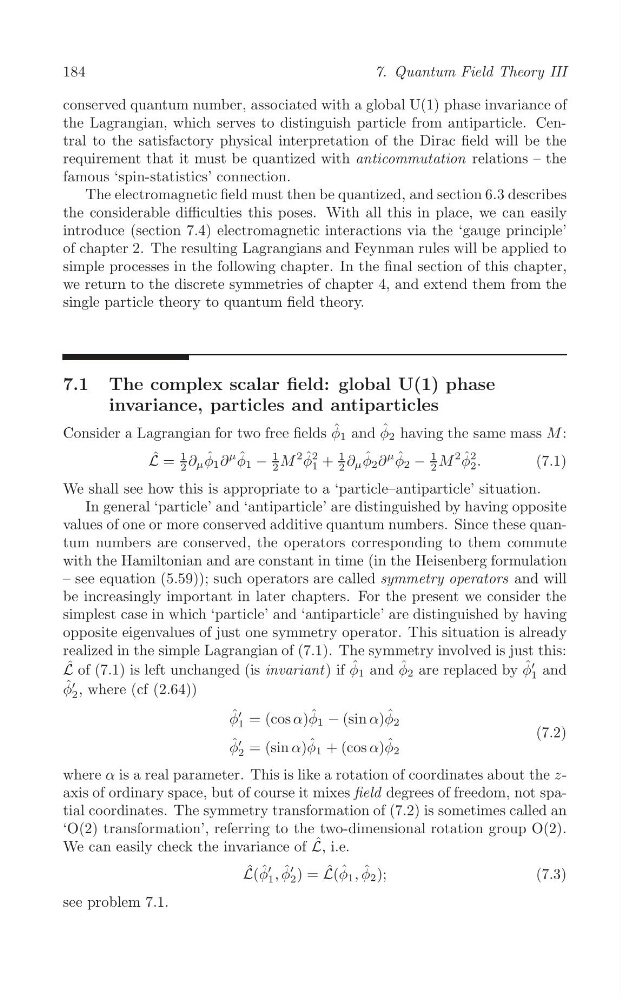
Consider a Lagrangian for two free fields φ ˆ 1 and φ ˆ 2 having the same mass M :
ˆ 1 φ ˆ 1 ∂
μ φ ˆ 1 −
1 M
2 φ ˆ 2
L =
1 +
1 ∂ μ φ ˆ 2 ∂
μ φ ˆ 2 −
1 M
2 φ ˆ 2
2 .
(7.1)
∂ μ
2
2
2
2
We shall see how this is appropriate to a ‘particle–antiparticle’ situation.
In general ‘particle’ and ‘antiparticle’ are distinguished by having opposite
values of one or more conserved additive quantum numbers. Since these quantum numbers are conserved, the operators corresponding to them commute
with the Hamiltonian and are constant in time (in the Heisenberg formulation
– see equation (5.59)); such operators are called symmetry operators and will
be increasingly important in later chapters. For the present we consider the
simplest case in which ‘particle’ and ‘antiparticle’ are distinguished by having
opposite eigenvalues of just one symmetry operator. This situation is already
realized in the simple Lagrangian of (7.1). The symmetry involved is just this:
L ˆ of (7.1) is left unchanged (is invariant ) if φ ˆ 1 and φ ˆ 2 are replaced by φ ˆ′
1 and
φ ˆ′
2 , where (cf (2.64))
φ ˆ′
1 = (cos α)φ ˆ 1 − (sin α)φ ˆ 2
(7.2)
φ ˆ ′
2 = (sin α)φ ˆ 1 + (cos α)φ ˆ 2
where α is a real parameter. This is like a rotation of coordinates about the zaxis of ordinary space, but of course it mixes field degrees of freedom, not spatial coordinates. The symmetry transformation of (7.2) is sometimes called an
‘O(2) transformation’, referring to the two-dimensional rotation group O(2).
We can easily check the invariance of L ˆ , i.e.
L ˆ (φ ˆ ′
1 , φ ˆ ′
2 ) = L ˆ (φ ˆ 1 , φ ˆ 2 );
(7.3)
see problem 7.1.
7. Quantum Field Theory III
conserved quantum number, associated with a global U(1) phase invariance of
the Lagrangian, which serves to distinguish particle from antiparticle. Central to the satisfactory physical interpretation of the Dirac field will be the
requirement that it must be quantized with anticommutation relations – the
famous ‘spin-statistics’ connection.
The electromagnetic field must then be quantized, and section 6.3 describes
the considerable difficulties this poses. With all this in place, we can easily
introduce (section 7.4) electromagnetic interactions via the ‘gauge principle’
of chapter 2. The resulting Lagrangians and Feynman rules will be applied to
simple processes in the following chapter. In the final section of this chapter,
we return to the discrete symmetries of chapter 4, and extend them from the
single particle theory to quantum field theory.
7.1 The complex scalar field: global U(1) phase
invariance, particles and antiparticles
Consider a Lagrangian for two free fields φ ˆ 1 and φ ˆ 2 having the same mass M :
ˆ 1 φ ˆ 1 ∂
μ φ ˆ 1 −
1 M
2 φ ˆ 2
L =
1 +
1 ∂ μ φ ˆ 2 ∂
μ φ ˆ 2 −
1 M
2 φ ˆ 2
2 .
(7.1)
∂ μ
2
2
2
2
We shall see how this is appropriate to a ‘particle–antiparticle’ situation.
In general ‘particle’ and ‘antiparticle’ are distinguished by having opposite
values of one or more conserved additive quantum numbers. Since these quantum numbers are conserved, the operators corresponding to them commute
with the Hamiltonian and are constant in time (in the Heisenberg formulation
– see equation (5.59)); such operators are called symmetry operators and will
be increasingly important in later chapters. For the present we consider the
simplest case in which ‘particle’ and ‘antiparticle’ are distinguished by having
opposite eigenvalues of just one symmetry operator. This situation is already
realized in the simple Lagrangian of (7.1). The symmetry involved is just this:
L ˆ of (7.1) is left unchanged (is invariant ) if φ ˆ 1 and φ ˆ 2 are replaced by φ ˆ′
1 and
φ ˆ′
2 , where (cf (2.64))
φ ˆ′
1 = (cos α)φ ˆ 1 − (sin α)φ ˆ 2
(7.2)
φ ˆ ′
2 = (sin α)φ ˆ 1 + (cos α)φ ˆ 2
where α is a real parameter. This is like a rotation of coordinates about the zaxis of ordinary space, but of course it mixes field degrees of freedom, not spatial coordinates. The symmetry transformation of (7.2) is sometimes called an
‘O(2) transformation’, referring to the two-dimensional rotation group O(2).
We can easily check the invariance of L ˆ , i.e.
L ˆ (φ ˆ ′
1 , φ ˆ ′
2 ) = L ˆ (φ ˆ 1 , φ ˆ 2 );
(7.3)
see problem 7.1.