

168
6. Quantum Field Theory II: Interacting Scalar Fields
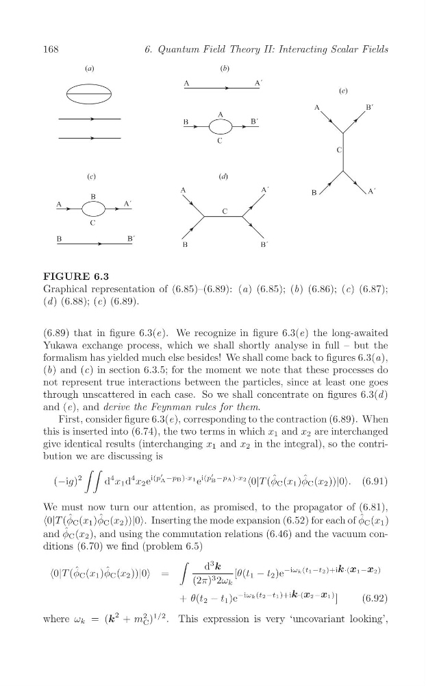
FIGURE 6.3
Graphical representation of (6.85)–(6.89): (a) (6.85); (b) (6.86); (c) (6.87);
(d ) (6.88); (e) (6.89).
(6.89) that in figure 6.3(e). We recognize in figure 6.3(e) the long-awaited
Yukawa exchange process, which we shall shortly analyse in full – but the
formalism has yielded much else besides! We shall come back to figures 6.3(a),
(b) and (c) in section 6.3.5; for the moment we note that these processes do
not represent true interactions between the particles, since at least one goes
through unscattered in each case. So we shall concentrate on figures 6.3(d )
and (e), and derive the Feynman rules for them.
First, consider figure 6.3(e), corresponding to the contraction (6.89). When
this is inserted into (6.74), the two terms in which x 1 and x 2 are interchanged
give identical results (interchanging x 1 and x 2 in the integral), so the contribution we are discussing is
∫ ∫
i(p −pB)·x1 i(p
A
B
(−ig)
2
d
4 x 1 d
4 x 2 e
'
e
' −pA)·x2
<0|T (φ ˆ C (x 1 )φ ˆ C (x 2 ))|0>. (6.91)
We must now turn our attention, as promised, to the propagator of (6.81),
<0|T (φ ˆ C (x 1 )φ ˆ C (x 2 ))|0>. Inserting the mode expansion (6.52) for each of φ ˆ C (x 1 )
and φ ˆ C (x 2 ), and using the commutation relations (6.46) and the vacuum conditions (6.70) we find (problem 6.5)
∫
d
3
k
<0|T (φ ˆ C (x 1 )φ ˆ C (x 2 ))|0> =
[θ(t 1 − t 2 )e
−iω k (t1−t2 )+ik·(x1−x2)
(2π) 3 2ω k
+ θ(t 2 − t 1 )e
−iω k (t2−t1 )+ik·(x2 −x1 ) ]
(6.92)
2 )
1/2
where ω k = (k
2 + m
. This expression is very ‘uncovariant looking’,
C
6. Quantum Field Theory II: Interacting Scalar Fields
FIGURE 6.3
Graphical representation of (6.85)–(6.89): (a) (6.85); (b) (6.86); (c) (6.87);
(d ) (6.88); (e) (6.89).
(6.89) that in figure 6.3(e). We recognize in figure 6.3(e) the long-awaited
Yukawa exchange process, which we shall shortly analyse in full – but the
formalism has yielded much else besides! We shall come back to figures 6.3(a),
(b) and (c) in section 6.3.5; for the moment we note that these processes do
not represent true interactions between the particles, since at least one goes
through unscattered in each case. So we shall concentrate on figures 6.3(d )
and (e), and derive the Feynman rules for them.
First, consider figure 6.3(e), corresponding to the contraction (6.89). When
this is inserted into (6.74), the two terms in which x 1 and x 2 are interchanged
give identical results (interchanging x 1 and x 2 in the integral), so the contribution we are discussing is
∫ ∫
i(p −pB)·x1 i(p
A
B
(−ig)
2
d
4 x 1 d
4 x 2 e
'
e
' −pA)·x2
<0|T (φ ˆ C (x 1 )φ ˆ C (x 2 ))|0>. (6.91)
We must now turn our attention, as promised, to the propagator of (6.81),
<0|T (φ ˆ C (x 1 )φ ˆ C (x 2 ))|0>. Inserting the mode expansion (6.52) for each of φ ˆ C (x 1 )
and φ ˆ C (x 2 ), and using the commutation relations (6.46) and the vacuum conditions (6.70) we find (problem 6.5)
∫
d
3
k
<0|T (φ ˆ C (x 1 )φ ˆ C (x 2 ))|0> =
[θ(t 1 − t 2 )e
−iω k (t1−t2 )+ik·(x1−x2)
(2π) 3 2ω k
+ θ(t 2 − t 1 )e
−iω k (t2−t1 )+ik·(x2 −x1 ) ]
(6.92)
2 )
1/2
where ω k = (k
2 + m
. This expression is very ‘uncovariant looking’,
C