

160
6. Quantum Field Theory II: Interacting Scalar Fields
such one-particle states, and zero for all other states. The normalization
choice (6.49) corresponds (see comment (5) in section 5.2.5) to a wavefunction
normalization of 2E i particles per unit volume.
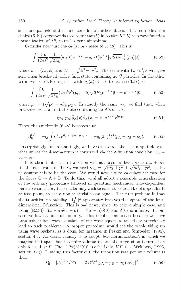
Consider now just the φ ˆ C (x)|p C > piece of (6.48). This is
∫ d
3
k
√
1
†
†
√
[ˆ a C (k)e
−ik·x + ˆ
a (k)e
ik·x ] 2E C a ˆ (p C )|0>
(6.52)
C
C
(2π) 3 2E k
√
k
2
2
where k = (E k , k) and E k =
+ m . The term with two ˆ
a
† ’s will give
C
C
zero when bracketed with a final state containing no C particles. In the other
term, we use (6.46) together with ˆ
a C (k)|0> = 0 to reduce (6.52) to
∫ d
3
k
√
1
√
(2π)
3 δ
3 (p C − k) 2E C e
−ik·x
|0> = e
−ipC ·x
|0>
(6.53)
(2π) 3 2E k
√
2
2
where p C = ( p + m C , p C ). In exactly the same way we find that, when
C
bracketed with an initial state containing no A’s or B’s,
ipA ·x ipB ·x
e
.
(6.54)
Hence the amplitude (6.48) becomes just
∫
(1)
d
4
i(pA+pB−pC)·x
A = −ig
xe
= −ig(2π)
4 δ
4 (p A + p B − p C ).
(6.55)
fi
Unsurprisingly, but reassuringly, we have discovered that the amplitude vanishes unless the 4-momentum is conserved via the δ-function condition: p C =
p A + p B .
It is clear that such a transition will not occur unless m C > m A + m B
√
√
2
2
(in the rest frame of the C, we need m C = m + p 2 + m + p 2 ), so let
A
B
us assume this to be the case. We would now like to calculate the rate for
the decay C → A + B. To do this, we shall adopt a plausible generalization
of the ordinary procedure followed in quantum mechanical time-dependent
perturbation theory (the reader may wish to consult section H.3 of appendix H
at this point, to see a non-relativistic analogue). The first problem is that
(1)
the transition probability |A |
2 apparently involves the square of the fourfi
dimensional δ-function. This is bad news, since (to take a simple case, and
using (E.53)) δ(x − a)δ(x − a) = δ(x − a)δ(0) and δ(0) is infinite. In our
case we have a four-fold infinity. This trouble has arisen because we have
been using plane-wave solutions of our wave equation, and these notoriously
lead to such problems. A proper procedure would set the whole thing up
using wave packets, as is done, for instance, in Peskin and Schroeder (1995),
section 4.5. An easier remedy is to adopt ‘box normalization’, in which we
imagine that space has the finite volume V , and the interaction is turned on
only for a time T . Then ‘(2π)
4 δ
4 (0)’ is effectively ‘V T ’ (see Weinberg (1995,
section 3.4)). Dividing this factor out, the transition rate per unit volume is
then
(1)
P ˙ fi = |A fi |
2 /V T = (2π)
4 δ
4 (p A + p B − p C )|M fi |
2
(6.56)
6. Quantum Field Theory II: Interacting Scalar Fields
such one-particle states, and zero for all other states. The normalization
choice (6.49) corresponds (see comment (5) in section 5.2.5) to a wavefunction
normalization of 2E i particles per unit volume.
Consider now just the φ ˆ C (x)|p C > piece of (6.48). This is
∫ d
3
k
√
1
†
†
√
[ˆ a C (k)e
−ik·x + ˆ
a (k)e
ik·x ] 2E C a ˆ (p C )|0>
(6.52)
C
C
(2π) 3 2E k
√
k
2
2
where k = (E k , k) and E k =
+ m . The term with two ˆ
a
† ’s will give
C
C
zero when bracketed with a final state containing no C particles. In the other
term, we use (6.46) together with ˆ
a C (k)|0> = 0 to reduce (6.52) to
∫ d
3
k
√
1
√
(2π)
3 δ
3 (p C − k) 2E C e
−ik·x
|0> = e
−ipC ·x
|0>
(6.53)
(2π) 3 2E k
√
2
2
where p C = ( p + m C , p C ). In exactly the same way we find that, when
C
bracketed with an initial state containing no A’s or B’s,
ipA ·x ipB ·x
e
.
(6.54)
Hence the amplitude (6.48) becomes just
∫
(1)
d
4
i(pA+pB−pC)·x
A = −ig
xe
= −ig(2π)
4 δ
4 (p A + p B − p C ).
(6.55)
fi
Unsurprisingly, but reassuringly, we have discovered that the amplitude vanishes unless the 4-momentum is conserved via the δ-function condition: p C =
p A + p B .
It is clear that such a transition will not occur unless m C > m A + m B
√
√
2
2
(in the rest frame of the C, we need m C = m + p 2 + m + p 2 ), so let
A
B
us assume this to be the case. We would now like to calculate the rate for
the decay C → A + B. To do this, we shall adopt a plausible generalization
of the ordinary procedure followed in quantum mechanical time-dependent
perturbation theory (the reader may wish to consult section H.3 of appendix H
at this point, to see a non-relativistic analogue). The first problem is that
(1)
the transition probability |A |
2 apparently involves the square of the fourfi
dimensional δ-function. This is bad news, since (to take a simple case, and
using (E.53)) δ(x − a)δ(x − a) = δ(x − a)δ(0) and δ(0) is infinite. In our
case we have a four-fold infinity. This trouble has arisen because we have
been using plane-wave solutions of our wave equation, and these notoriously
lead to such problems. A proper procedure would set the whole thing up
using wave packets, as is done, for instance, in Peskin and Schroeder (1995),
section 4.5. An easier remedy is to adopt ‘box normalization’, in which we
imagine that space has the finite volume V , and the interaction is turned on
only for a time T . Then ‘(2π)
4 δ
4 (0)’ is effectively ‘V T ’ (see Weinberg (1995,
section 3.4)). Dividing this factor out, the transition rate per unit volume is
then
(1)
P ˙ fi = |A fi |
2 /V T = (2π)
4 δ
4 (p A + p B − p C )|M fi |
2
(6.56)