

139
5.2. The quantum field: (ii) Lagrange–Hamilton formulation
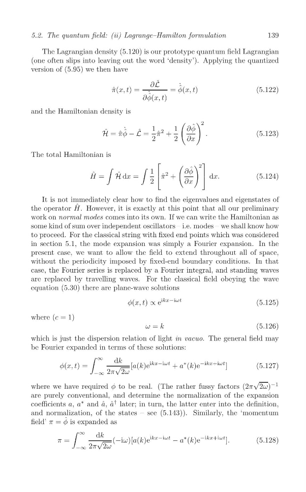
The Lagrangian density (5.120) is our prototype quantum field Lagrangian
(one often slips into leaving out the word ‘density’). Applying the quantized
version of (5.95) we then have
∂L ˆ
ˆ ˙
π ˆ(x, t) =
= φ(x, t)
(5.122)
˙
ˆ
∂φ(x, t)
and the Hamiltonian density is
( ) 2
˙
1
1 ∂φ ˆ
H ˆ = ˆ
πφ ˆ − L ˆ = π ˆ
2 +
.
(5.123)
2
2 ∂x
The total Hamiltonian is
[
( ) 2
]
∫
∫ 1
∂φ ˆ
H ˆ = H ˆ dx =
| π ˆ
2 +
| dx.
(5.124)
2
∂x
It is not immediately clear how to find the eigenvalues and eigenstates of
the operator H ˆ . However, it is exactly at this point that all our preliminary
work on normal modes comes into its own. If we can write the Hamiltonian as
some kind of sum over independent oscillators – i.e. modes – we shall know how
to proceed. For the classical string with fixed end points which was considered
in section 5.1, the mode expansion was simply a Fourier expansion. In the
present case, we want to allow the field to extend throughout all of space,
without the periodicity imposed by fixed-end boundary conditions. In that
case, the Fourier series is replaced by a Fourier integral, and standing waves
are replaced by travelling waves. For the classical field obeying the wave
equation (5.30) there are plane-wave solutions
ikx−iωt
φ(x, t) ∝ e
(5.125)
where (c = 1)
ω = k
(5.126)
which is just the dispersion relation of light in vacuo. The general field may
be Fourier expanded in terms of these solutions:
∫ ∞
φ(x, t) =
d
√
k [a(k)e
ikx−iωt + a
∗ (k)e
−ikx+iωt ]
(5.127)
−∞ 2π 2ω
√
where we have required φ to be real. (The rather fussy factors (2π 2ω)
−1
are purely conventional, and determine the normalization of the expansion
coefficients a, a
∗ and ˆ
a, ˆ
a
† later; in turn, the latter enter into the definition,
and normalization, of the states – see (5.143)). Similarly, the ‘momentum
˙
field’ π = φ is expanded as
∫ ∞
π =
d
√
k (−iω)[a(k)e
ikx−iωt
− a
∗ (k)e
−ikx+iωt ].
(5.128)
−∞ 2π 2ω
5.2. The quantum field: (ii) Lagrange–Hamilton formulation
The Lagrangian density (5.120) is our prototype quantum field Lagrangian
(one often slips into leaving out the word ‘density’). Applying the quantized
version of (5.95) we then have
∂L ˆ
ˆ ˙
π ˆ(x, t) =
= φ(x, t)
(5.122)
˙
ˆ
∂φ(x, t)
and the Hamiltonian density is
( ) 2
˙
1
1 ∂φ ˆ
H ˆ = ˆ
πφ ˆ − L ˆ = π ˆ
2 +
.
(5.123)
2
2 ∂x
The total Hamiltonian is
[
( ) 2
]
∫
∫ 1
∂φ ˆ
H ˆ = H ˆ dx =
| π ˆ
2 +
| dx.
(5.124)
2
∂x
It is not immediately clear how to find the eigenvalues and eigenstates of
the operator H ˆ . However, it is exactly at this point that all our preliminary
work on normal modes comes into its own. If we can write the Hamiltonian as
some kind of sum over independent oscillators – i.e. modes – we shall know how
to proceed. For the classical string with fixed end points which was considered
in section 5.1, the mode expansion was simply a Fourier expansion. In the
present case, we want to allow the field to extend throughout all of space,
without the periodicity imposed by fixed-end boundary conditions. In that
case, the Fourier series is replaced by a Fourier integral, and standing waves
are replaced by travelling waves. For the classical field obeying the wave
equation (5.30) there are plane-wave solutions
ikx−iωt
φ(x, t) ∝ e
(5.125)
where (c = 1)
ω = k
(5.126)
which is just the dispersion relation of light in vacuo. The general field may
be Fourier expanded in terms of these solutions:
∫ ∞
φ(x, t) =
d
√
k [a(k)e
ikx−iωt + a
∗ (k)e
−ikx+iωt ]
(5.127)
−∞ 2π 2ω
√
where we have required φ to be real. (The rather fussy factors (2π 2ω)
−1
are purely conventional, and determine the normalization of the expansion
coefficients a, a
∗ and ˆ
a, ˆ
a
† later; in turn, the latter enter into the definition,
and normalization, of the states – see (5.143)). Similarly, the ‘momentum
˙
field’ π = φ is expanded as
∫ ∞
π =
d
√
k (−iω)[a(k)e
ikx−iωt
− a
∗ (k)e
−ikx+iωt ].
(5.128)
−∞ 2π 2ω