

138
5. Quantum Field Theory I: The Free Scalar Field
also note that (5.114) is between operators at equal times. The continuum
generalization of the δ rs symbol is the Dirac δ function, δ(x − y), with the
properties
∫ ∞
−∞ δ(x) dx = 1
(5.115)
∫ ∞ δ(x − y)f (x) dx = f (y)
(5.116)
−∞
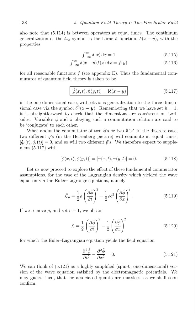
for all reasonable functions f (see appendix E). Thus the fundamental commutator of quantum field theory is taken to be
[φ ˆ (x, t), π ˆ(y, t)] = iδ(x − y)
(5.117)
in the one-dimensional case, with obvious generalization to the three-dimensional case via the symbol δ
3 (x − y). Remembering that we have set ħ = 1,
it is straightforward to check that the dimensions are consistent on both
sides. Variables φ ˆ and ˆ
π obeying such a commutation relation are said to
be ‘conjugate’ to each other.
What about the commutator of two φ ˆ ’s or two ˆ
π’s? In the discrete case,
two different ˆ
q’s (in the Heisenberg picture) will commute at equal times,
[ˆ q r (t), q ˆ s (t)] = 0, and so will two different ˆ
p’s. We therefore expect to supplement (5.117) with
[φ ˆ (x, t), φ ˆ (y, t)] = [ˆ π(x, t), π ˆ(y, t)] = 0.
(5.118)
Let us now proceed to explore the effect of these fundamental commutator
assumptions, for the case of the Lagrangian density which yielded the wave
equation via the Euler–Lagrange equations, namely
( ) 2
( ) 2
1
∂φ ˆ
1
∂φ ˆ
ˆ
L ρ = ρ
− ρc
2
.
(5.119)
2
∂t
2
∂x
If we remove ρ, and set c = 1, we obtain
( ) 2
( ) 2
1 ∂φ ˆ
1 ∂φ ˆ
ˆ
L =
−
(5.120)
2 ∂t
2 ∂x
for which the Euler–Lagrangian equation yields the field equation
∂
2 ˆ ∂
2 ˆ
φ
φ
−
= 0.
(5.121)
∂t 2
∂x 2
We can think of (5.121) as a highly simplified (spin-0, one-dimensional) version of the wave equation satisfied by the electromagnetic potentials. We
may guess, then, that the associated quanta are massless, as we shall soon
confirm.
5. Quantum Field Theory I: The Free Scalar Field
also note that (5.114) is between operators at equal times. The continuum
generalization of the δ rs symbol is the Dirac δ function, δ(x − y), with the
properties
∫ ∞
−∞ δ(x) dx = 1
(5.115)
∫ ∞ δ(x − y)f (x) dx = f (y)
(5.116)
−∞
for all reasonable functions f (see appendix E). Thus the fundamental commutator of quantum field theory is taken to be
[φ ˆ (x, t), π ˆ(y, t)] = iδ(x − y)
(5.117)
in the one-dimensional case, with obvious generalization to the three-dimensional case via the symbol δ
3 (x − y). Remembering that we have set ħ = 1,
it is straightforward to check that the dimensions are consistent on both
sides. Variables φ ˆ and ˆ
π obeying such a commutation relation are said to
be ‘conjugate’ to each other.
What about the commutator of two φ ˆ ’s or two ˆ
π’s? In the discrete case,
two different ˆ
q’s (in the Heisenberg picture) will commute at equal times,
[ˆ q r (t), q ˆ s (t)] = 0, and so will two different ˆ
p’s. We therefore expect to supplement (5.117) with
[φ ˆ (x, t), φ ˆ (y, t)] = [ˆ π(x, t), π ˆ(y, t)] = 0.
(5.118)
Let us now proceed to explore the effect of these fundamental commutator
assumptions, for the case of the Lagrangian density which yielded the wave
equation via the Euler–Lagrange equations, namely
( ) 2
( ) 2
1
∂φ ˆ
1
∂φ ˆ
ˆ
L ρ = ρ
− ρc
2
.
(5.119)
2
∂t
2
∂x
If we remove ρ, and set c = 1, we obtain
( ) 2
( ) 2
1 ∂φ ˆ
1 ∂φ ˆ
ˆ
L =
−
(5.120)
2 ∂t
2 ∂x
for which the Euler–Lagrangian equation yields the field equation
∂
2 ˆ ∂
2 ˆ
φ
φ
−
= 0.
(5.121)
∂t 2
∂x 2
We can think of (5.121) as a highly simplified (spin-0, one-dimensional) version of the wave equation satisfied by the electromagnetic potentials. We
may guess, then, that the associated quanta are massless, as we shall soon
confirm.