

123
5.1. The quantum field: (i) descriptive
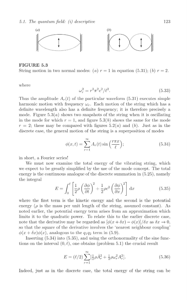
FIGURE 5.3
String motion in two normal modes: (a) r = 1 in equation (5.31); (b) r = 2.
where
ω
2 = r
2 π
2 c
2 /e
2 .
(5.33)
r
Thus the amplitude A r (t) of the particular waveform (5.31) executes simple
harmonic motion with frequency ω r . Each motion of the string which has a
definite wavelength also has a definite frequency; it is therefore precisely a
mode. Figure 5.3(a) shows two snapshots of the string when it is oscillating
in the mode for which r = 1, and figure 5.3(b) shows the same for the mode
r = 2; these may be compared with figures 5.2(a) and (b). Just as in the
discrete case, the general motion of the string is a superposition of modes
∞
∑
(
)
rπx
φ(x, t) =
A r (t) sin
;
(5.34)
e
r=1
in short, a Fourier series!
We must now examine the total energy of the vibrating string, which
we expect to be greatly simplified by the use of the mode concept. The total
energy is the continuous analogue of the discrete summation in (5.25), namely
the integral
∫ [ ( ) 2
( ) 2
]
e 1
∂φ
1
∂φ
E =
ρ
+ ρc
2
dx
(5.35)
2
∂t
2
∂x
0
where the first term is the kinetic energy and the second is the potential
energy (ρ is the mass per unit length of the string, assumed constant). As
noted earlier, the potential energy term arises from an approximation which
limits it to the quadratic power. To relate this to the earlier discrete case,
note that the derivative may be regarded as [φ(x + δx) − φ(x)]/δx as δx → 0,
so that the square of the derivative involves the ‘nearest neighbour coupling’
φ(x + δx)φ(x), analogous to the q 1 q 2 term in (5.9).
Inserting (5.34) into (5.35), and using the orthonormality of the sine functions on the interval (0, e), one obtains (problem 5.1) the crucial result
∞
∑
1
E = (e/2)
[
1 ρA ˙ 2 + ρω
2 A
2 ].
(5.36)
2
r
2
r r
r=1
Indeed, just as in the discrete case, the total energy of the string can be
5.1. The quantum field: (i) descriptive
FIGURE 5.3
String motion in two normal modes: (a) r = 1 in equation (5.31); (b) r = 2.
where
ω
2 = r
2 π
2 c
2 /e
2 .
(5.33)
r
Thus the amplitude A r (t) of the particular waveform (5.31) executes simple
harmonic motion with frequency ω r . Each motion of the string which has a
definite wavelength also has a definite frequency; it is therefore precisely a
mode. Figure 5.3(a) shows two snapshots of the string when it is oscillating
in the mode for which r = 1, and figure 5.3(b) shows the same for the mode
r = 2; these may be compared with figures 5.2(a) and (b). Just as in the
discrete case, the general motion of the string is a superposition of modes
∞
∑
(
)
rπx
φ(x, t) =
A r (t) sin
;
(5.34)
e
r=1
in short, a Fourier series!
We must now examine the total energy of the vibrating string, which
we expect to be greatly simplified by the use of the mode concept. The total
energy is the continuous analogue of the discrete summation in (5.25), namely
the integral
∫ [ ( ) 2
( ) 2
]
e 1
∂φ
1
∂φ
E =
ρ
+ ρc
2
dx
(5.35)
2
∂t
2
∂x
0
where the first term is the kinetic energy and the second is the potential
energy (ρ is the mass per unit length of the string, assumed constant). As
noted earlier, the potential energy term arises from an approximation which
limits it to the quadratic power. To relate this to the earlier discrete case,
note that the derivative may be regarded as [φ(x + δx) − φ(x)]/δx as δx → 0,
so that the square of the derivative involves the ‘nearest neighbour coupling’
φ(x + δx)φ(x), analogous to the q 1 q 2 term in (5.9).
Inserting (5.34) into (5.35), and using the orthonormality of the sine functions on the interval (0, e), one obtains (problem 5.1) the crucial result
∞
∑
1
E = (e/2)
[
1 ρA ˙ 2 + ρω
2 A
2 ].
(5.36)
2
r
2
r r
r=1
Indeed, just as in the discrete case, the total energy of the string can be