

122
5. Quantum Field Theory I: The Free Scalar Field
are n r quanta present’. For the state characterized by (n 1 , n 2 ,. . ., n N ) there
are n 1 quanta of mode 1 (frequency ω 1 ), n 2 of mode 2, . . . and n N of mode N .
Note particularly that although the number of modes N is fixed, the values of
the n r ’s are unrestricted, except insofar as the total energy is fixed. Thus we
are moving from a ‘fixed number’ picture (N degrees of freedom) to a ‘variable number’ picture (the n r ’s restricted only by the total energy constraint
(5.29)). In the case of a real solid, these quanta of vibrational energy are
called phonons. We summarize the point we have reached by the important
statement that a phonon is an elementary quantum of vibrational excitation.
Now we take one step backward in order, afterwards, to take two steps
forward. We return to the classical mechanical model with N harmonically
interacting degrees of freedom. It is possible to imagine increasing the number N to infinity, and decreasing the interatomic spacing a to zero, in such a
way that the product N a stays finite, say N a = e. We then have a classical
continuous system – for example a string of length e. (We stay in one dimension for simplicity.) The transverse vibrations of this string are now described
by a f ield φ(x, t), where at each point x of the string φ(x, t) measures the displacement from equilibrium, at the time t, of a small element of string around
the point x. Thus we have passed from a system described by a discrete number of degrees of freedom, q r (t) or Q r (t), to one described by a continuous
degree of freedom, the displacement field φ(x, t). The discrete suffix r has
become the continuous argument x – and to prepare for later abstraction, we
have denoted the displacement by φ(x, t) rather than, say, q(x, t).
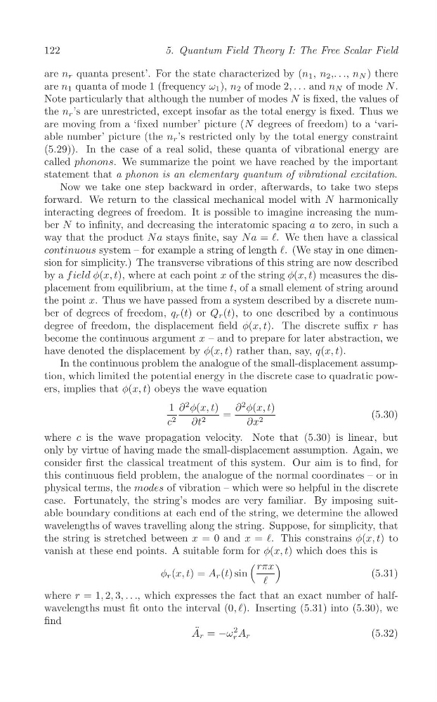
In the continuous problem the analogue of the small-displacement assumption, which limited the potential energy in the discrete case to quadratic powers, implies that φ(x, t) obeys the wave equation
1 ∂
2 φ(x, t)
∂
2 φ(x, t)
=
(5.30)
c 2 ∂t 2
∂x 2
where c is the wave propagation velocity. Note that (5.30) is linear, but
only by virtue of having made the small-displacement assumption. Again, we
consider first the classical treatment of this system. Our aim is to find, for
this continuous field problem, the analogue of the normal coordinates – or in
physical terms, the modes of vibration – which were so helpful in the discrete
case. Fortunately, the string’s modes are very familiar. By imposing suitable boundary conditions at each end of the string, we determine the allowed
wavelengths of waves travelling along the string. Suppose, for simplicity, that
the string is stretched between x = 0 and x = e. This constrains φ(x, t) to
vanish at these end points. A suitable form for φ(x, t) which does this is
(
)
rπx
φ r (x, t) = A r (t) sin
(5.31)
e
where r = 1, 2, 3, . . ., which expresses the fact that an exact number of halfwavelengths must fit onto the interval (0, e). Inserting (5.31) into (5.30), we
find
¨
A r = −ω
2 A r
(5.32)
r
5. Quantum Field Theory I: The Free Scalar Field
are n r quanta present’. For the state characterized by (n 1 , n 2 ,. . ., n N ) there
are n 1 quanta of mode 1 (frequency ω 1 ), n 2 of mode 2, . . . and n N of mode N .
Note particularly that although the number of modes N is fixed, the values of
the n r ’s are unrestricted, except insofar as the total energy is fixed. Thus we
are moving from a ‘fixed number’ picture (N degrees of freedom) to a ‘variable number’ picture (the n r ’s restricted only by the total energy constraint
(5.29)). In the case of a real solid, these quanta of vibrational energy are
called phonons. We summarize the point we have reached by the important
statement that a phonon is an elementary quantum of vibrational excitation.
Now we take one step backward in order, afterwards, to take two steps
forward. We return to the classical mechanical model with N harmonically
interacting degrees of freedom. It is possible to imagine increasing the number N to infinity, and decreasing the interatomic spacing a to zero, in such a
way that the product N a stays finite, say N a = e. We then have a classical
continuous system – for example a string of length e. (We stay in one dimension for simplicity.) The transverse vibrations of this string are now described
by a f ield φ(x, t), where at each point x of the string φ(x, t) measures the displacement from equilibrium, at the time t, of a small element of string around
the point x. Thus we have passed from a system described by a discrete number of degrees of freedom, q r (t) or Q r (t), to one described by a continuous
degree of freedom, the displacement field φ(x, t). The discrete suffix r has
become the continuous argument x – and to prepare for later abstraction, we
have denoted the displacement by φ(x, t) rather than, say, q(x, t).
In the continuous problem the analogue of the small-displacement assumption, which limited the potential energy in the discrete case to quadratic powers, implies that φ(x, t) obeys the wave equation
1 ∂
2 φ(x, t)
∂
2 φ(x, t)
=
(5.30)
c 2 ∂t 2
∂x 2
where c is the wave propagation velocity. Note that (5.30) is linear, but
only by virtue of having made the small-displacement assumption. Again, we
consider first the classical treatment of this system. Our aim is to find, for
this continuous field problem, the analogue of the normal coordinates – or in
physical terms, the modes of vibration – which were so helpful in the discrete
case. Fortunately, the string’s modes are very familiar. By imposing suitable boundary conditions at each end of the string, we determine the allowed
wavelengths of waves travelling along the string. Suppose, for simplicity, that
the string is stretched between x = 0 and x = e. This constrains φ(x, t) to
vanish at these end points. A suitable form for φ(x, t) which does this is
(
)
rπx
φ r (x, t) = A r (t) sin
(5.31)
e
where r = 1, 2, 3, . . ., which expresses the fact that an exact number of halfwavelengths must fit onto the interval (0, e). Inserting (5.31) into (5.30), we
find
¨
A r = −ω
2 A r
(5.32)
r