

100
4. Lorentz Transformations and Discrete Symmetries
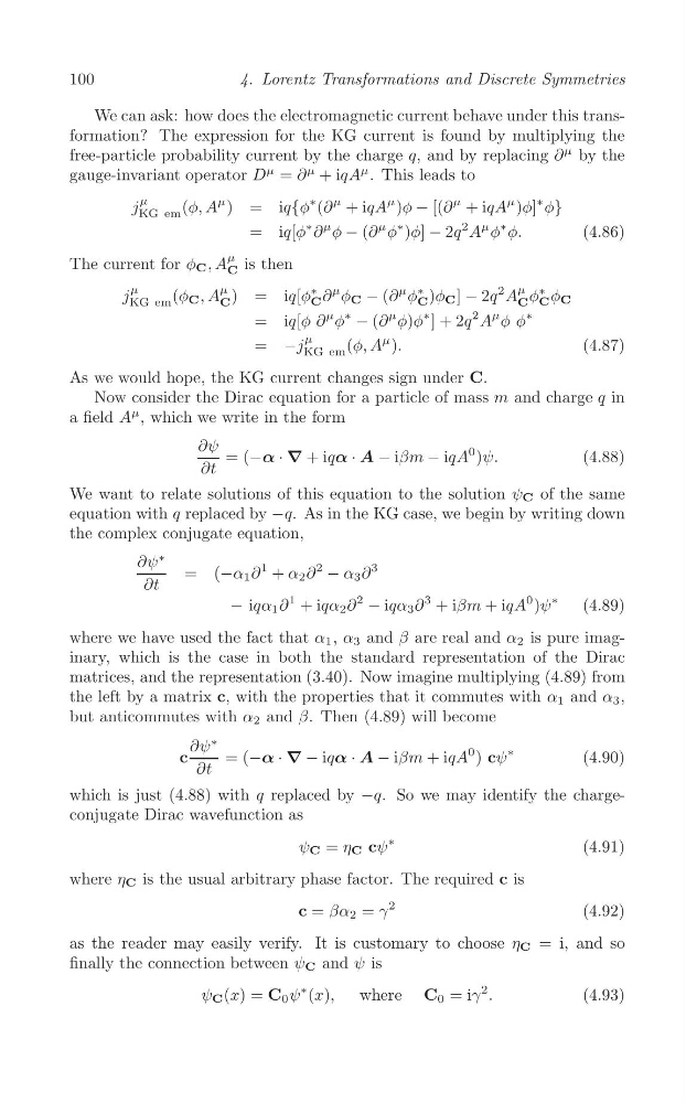
We can ask: how does the electromagnetic current behave under this transformation? The expression for the KG current is found by multiplying the
free-particle probability current by the charge q, and by replacing ∂
μ by the
gauge-invariant operator D
μ = ∂
μ + iqA
μ . This leads to
j
μ
(φ, A
μ ) = iq{φ
∗ (∂
μ + iqA
μ )φ − [(∂
μ + iqA
μ )φ]
∗ φ}
KG em
= iq[φ
∗ ∂
μ φ − (∂
μ φ
∗ )φ] − 2q
2 A
μ φ
∗ φ.
(4.86)
μ
The current for φ C , A C is then
μ
μ
μ
j
(φ C , A
iq[φ
∗
C )φ C ] − 2q
2 A φ C
∗ φ C
) =
C ∂
μ φ C − (∂
μ φ
∗
KG em
C
C
= iq[φ ∂
μ φ
∗
− (∂
μ φ)φ
∗ ] + 2q
2 A
μ φ φ
∗
μ
= −j
(φ, A
μ ).
(4.87)
KG em
As we would hope, the KG current changes sign under C.
Now consider the Dirac equation for a particle of mass m and charge q in
a field A
μ , which we write in the form
∂ψ = (−α · ∇ + iqα · A − iβm − iqA
0 )ψ.
(4.88)
∂t
We want to relate solutions of this equation to the solution ψ C of the same
equation with q replaced by −q. As in the KG case, we begin by writing down
the complex conjugate equation,
∂ψ
∗
= (−α 1 ∂
1 + α 2 ∂
2
− α 3 ∂
3
∂t
− iqα 1 ∂
1 + iqα 2 ∂
2
− iqα 3 ∂
3 + iβm + iqA
0 )ψ
∗
(4.89)
where we have used the fact that α 1 , α 3 and β are real and α 2 is pure imaginary, which is the case in both the standard representation of the Dirac
matrices, and the representation (3.40). Now imagine multiplying (4.89) from
the left by a matrix c, with the properties that it commutes with α 1 and α 3 ,
but anticommutes with α 2 and β. Then (4.89) will become
∂ψ
∗
c
= (−α · ∇ − iqα · A − iβm + iqA
0 ) cψ
∗
(4.90)
∂t
which is just (4.88) with q replaced by −q. So we may identify the chargeconjugate Dirac wavefunction as
ψ C = η C cψ
∗
(4.91)
where η C is the usual arbitrary phase factor. The required c is
c = βα 2 = γ
2
(4.92)
as the reader may easily verify. It is customary to choose η C = i, and so
finally the connection between ψ C and ψ is
ψ C (x) = C 0 ψ
∗ (x),
where C 0 = iγ
2 .
(4.93)
4. Lorentz Transformations and Discrete Symmetries
We can ask: how does the electromagnetic current behave under this transformation? The expression for the KG current is found by multiplying the
free-particle probability current by the charge q, and by replacing ∂
μ by the
gauge-invariant operator D
μ = ∂
μ + iqA
μ . This leads to
j
μ
(φ, A
μ ) = iq{φ
∗ (∂
μ + iqA
μ )φ − [(∂
μ + iqA
μ )φ]
∗ φ}
KG em
= iq[φ
∗ ∂
μ φ − (∂
μ φ
∗ )φ] − 2q
2 A
μ φ
∗ φ.
(4.86)
μ
The current for φ C , A C is then
μ
μ
μ
j
(φ C , A
iq[φ
∗
C )φ C ] − 2q
2 A φ C
∗ φ C
) =
C ∂
μ φ C − (∂
μ φ
∗
KG em
C
C
= iq[φ ∂
μ φ
∗
− (∂
μ φ)φ
∗ ] + 2q
2 A
μ φ φ
∗
μ
= −j
(φ, A
μ ).
(4.87)
KG em
As we would hope, the KG current changes sign under C.
Now consider the Dirac equation for a particle of mass m and charge q in
a field A
μ , which we write in the form
∂ψ = (−α · ∇ + iqα · A − iβm − iqA
0 )ψ.
(4.88)
∂t
We want to relate solutions of this equation to the solution ψ C of the same
equation with q replaced by −q. As in the KG case, we begin by writing down
the complex conjugate equation,
∂ψ
∗
= (−α 1 ∂
1 + α 2 ∂
2
− α 3 ∂
3
∂t
− iqα 1 ∂
1 + iqα 2 ∂
2
− iqα 3 ∂
3 + iβm + iqA
0 )ψ
∗
(4.89)
where we have used the fact that α 1 , α 3 and β are real and α 2 is pure imaginary, which is the case in both the standard representation of the Dirac
matrices, and the representation (3.40). Now imagine multiplying (4.89) from
the left by a matrix c, with the properties that it commutes with α 1 and α 3 ,
but anticommutes with α 2 and β. Then (4.89) will become
∂ψ
∗
c
= (−α · ∇ − iqα · A − iβm + iqA
0 ) cψ
∗
(4.90)
∂t
which is just (4.88) with q replaced by −q. So we may identify the chargeconjugate Dirac wavefunction as
ψ C = η C cψ
∗
(4.91)
where η C is the usual arbitrary phase factor. The required c is
c = βα 2 = γ
2
(4.92)
as the reader may easily verify. It is customary to choose η C = i, and so
finally the connection between ψ C and ψ is
ψ C (x) = C 0 ψ
∗ (x),
where C 0 = iγ
2 .
(4.93)