

being misconstrued, statistically assessing data using the
parametric tests is a robust way to show that the results were
not due to chance. In this research, the t-test was employed
to assess whether the cumulative abnormal returns were
significantly different from zero, with the hypotheses being:
Ho: CAR during the event window are not statistically
different from zero.
H1: CAR during the event window are statistically different from zero.
The t-stat in both models (mean average and market
model) were significant at a 1% level of significance, from
which the research concluded that the results were indeed
significant and the null hypothesis was rejected. This would
suggest that the t-test has qualified both the mean average
and the market model; however, we must consider the fact
that one of these models was derived from another element
all together, the beta.
A major part of the research hinged on regressing and
obtaining beta which was then implemented in the market
model to obtain the expected returns, which were then used
to calculate the abnormal returns. Though the t-statistic
validated the significance of the beta obtained, a small
degree of positive serial correlation was detected, the Durbin
Watson statistic was just below 2 (at 1.924). It is also
noteworthy to mention the rather small adjusted R2 value of
0.0454, and this would indicate that the model had a weak
performance. The residual normality test would also suggest
that the normal distribution does not exist. The Jarque–Bera
probability was at 0.07 which is higher than the critical value
of 5% from which the null hypothesis of ‘normal distribution
exists’ would be rejected.
Additionally, a fixed effects test was carried out to test for
unobserved heterogeneity, for which the p-value from the F
test was significant at 5%. The null hypothesis of ‘observed
heterogeneity’ must be rejected meaning that there is
unobserved heterogeneity.
The robustness testing mentioned above poses a robustness concern, due to the extremely low R2 figure. Foreseeing
the challenges that could arise from estimating beta using the
market model, this research was conducted on two separate
models. The mean average return model provided a benchmark for which the market model could be assessed. As
quite a substantial number of academic literature has praised
the robustness of the simple average return model, it appears
it would be the right model to apply in this situation. The
fact that there are some robustness concerns with the estimation of beta, the mean average model managed to map out
the expected return and the subsequent abnormal returns.
Compared to these returns, the market model performed
extremely well, which has been visually represented on
Fig. 1.4. The two model’s abnormal returns are not only
synchronous with one another, but they both managed to
significantly assess and measure the abnormal returns during
the event in question.
Other concerns with the research include the model that
was applied to measure the abnormal returns. As exchange
rates are rather complicated to assess, a more suitable model
(other than the market model) could have been used. Though
multiple factor models could have been applied in the pursuit of more accurate results, past literature suggests that the
mean average model is just as effective as more complicated
models. Hence, the use of a more complex model was not
seen as a necessity in this regard, meaning that the market
model (using a single factor element) was employed and
alongside it, the mean average returns were utilized to
confirm the results at hand.
Moreover, there are other concerns with the estimation
period that was used to estimate beta and the standard
deviation for the abnormal returns. The date of the EU referendum was announced in February 2016, which also
coincides with the estimation period, which was used in this
research. As it was expected that the EU referendum date
announcement would have had an effect on the GBP’s value,
this information should have been considered in the analysis.
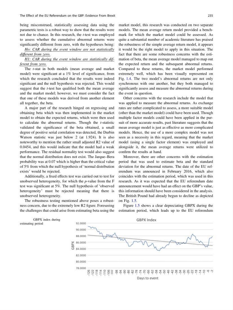
The British Pound had already begun to decline as depicted
on Fig. 1.5.
Figure 1.5 shows a clear depreciating GBPX during the
estimation period, which leads up to the EU referendum
Fig. 1.5 GBPX index during
estimating period
The Effect of the EU Referendum on the GBP: Evidence From Brexit
235
parametric tests is a robust way to show that the results were
not due to chance. In this research, the t-test was employed
to assess whether the cumulative abnormal returns were
significantly different from zero, with the hypotheses being:
Ho: CAR during the event window are not statistically
different from zero.
H1: CAR during the event window are statistically different from zero.
The t-stat in both models (mean average and market
model) were significant at a 1% level of significance, from
which the research concluded that the results were indeed
significant and the null hypothesis was rejected. This would
suggest that the t-test has qualified both the mean average
and the market model; however, we must consider the fact
that one of these models was derived from another element
all together, the beta.
A major part of the research hinged on regressing and
obtaining beta which was then implemented in the market
model to obtain the expected returns, which were then used
to calculate the abnormal returns. Though the t-statistic
validated the significance of the beta obtained, a small
degree of positive serial correlation was detected, the Durbin
Watson statistic was just below 2 (at 1.924). It is also
noteworthy to mention the rather small adjusted R2 value of
0.0454, and this would indicate that the model had a weak
performance. The residual normality test would also suggest
that the normal distribution does not exist. The Jarque–Bera
probability was at 0.07 which is higher than the critical value
of 5% from which the null hypothesis of ‘normal distribution
exists’ would be rejected.
Additionally, a fixed effects test was carried out to test for
unobserved heterogeneity, for which the p-value from the F
test was significant at 5%. The null hypothesis of ‘observed
heterogeneity’ must be rejected meaning that there is
unobserved heterogeneity.
The robustness testing mentioned above poses a robustness concern, due to the extremely low R2 figure. Foreseeing
the challenges that could arise from estimating beta using the
market model, this research was conducted on two separate
models. The mean average return model provided a benchmark for which the market model could be assessed. As
quite a substantial number of academic literature has praised
the robustness of the simple average return model, it appears
it would be the right model to apply in this situation. The
fact that there are some robustness concerns with the estimation of beta, the mean average model managed to map out
the expected return and the subsequent abnormal returns.
Compared to these returns, the market model performed
extremely well, which has been visually represented on
Fig. 1.4. The two model’s abnormal returns are not only
synchronous with one another, but they both managed to
significantly assess and measure the abnormal returns during
the event in question.
Other concerns with the research include the model that
was applied to measure the abnormal returns. As exchange
rates are rather complicated to assess, a more suitable model
(other than the market model) could have been used. Though
multiple factor models could have been applied in the pursuit of more accurate results, past literature suggests that the
mean average model is just as effective as more complicated
models. Hence, the use of a more complex model was not
seen as a necessity in this regard, meaning that the market
model (using a single factor element) was employed and
alongside it, the mean average returns were utilized to
confirm the results at hand.
Moreover, there are other concerns with the estimation
period that was used to estimate beta and the standard
deviation for the abnormal returns. The date of the EU referendum was announced in February 2016, which also
coincides with the estimation period, which was used in this
research. As it was expected that the EU referendum date
announcement would have had an effect on the GBP’s value,
this information should have been considered in the analysis.
The British Pound had already begun to decline as depicted
on Fig. 1.5.
Figure 1.5 shows a clear depreciating GBPX during the
estimation period, which leads up to the EU referendum
Fig. 1.5 GBPX index during
estimating period
The Effect of the EU Referendum on the GBP: Evidence From Brexit
235