

where the shear elastic modulus G
0 (ω) and the viscous modulus G
00 (ω) are the
inphase and out of phase components, respectively.
This stress response is interpreted as the Fourier transform of the stress relaxation
function G(t) of the quiescent state: G
0 (ω)=ω
Ð 1
0 G t
ð Þ sin ωt:dt, G
00 (ω)=ω
Ð 1
0 G t
ð Þ
cos ωt:dt . Under linear strain-stress conditions, the shear stress response does
reproduce the applied strain wave; i.e. it is a simple harmonic function of the applied
wave. G
0
> G
00 indicates a solid-like behavior, while G
00
> G
0 indicates a viscous or
flow behavior. Liquids and viscoelastic liquids are characterized by a flow behavior
at low frequency, typically within 0.1–10
2 Hz.
The surface interactions have a key role for the validity of the stress measurement.
In a conventional measurement (millimeter thickness sample probed using aluminum, stainless steel, or glass substrates), the dynamic relaxation spectrum of polymers
in the molten state exhibits, versus frequency, the typical Maxwell viscoelastic
response (Ferry 1961). At low frequencies, the response is depicted by a ω-scaling
decrease of the viscous modulus (G
00 ) and a ω
2
-scaling of the elastic modulus (G
0 ). G
0
being negligible compared to the viscous modulus (Fig. 5a bottom), the flow behavior
thus describes the frequency part where the viscous component becomes important.
The interception of the two curves defines the terminal time τ t , i.e., the largest time
before the material enters in a flow regime. This characteristic time is interpreted as the
longest molecular relaxation time (Rouse model).
Transducer
(transmitted torque)
Upper surface
Lower surface
Sample
Measure
Control
speed/
position
Control motor
speed
Motor
Bottom
fixture
Adhesion /
Friction/Slip
Adhesion /
Friction / Slip
Upper
fixture
F
Sensor:
Transform:
motion ->
tension
Torque:
Ω − Ω”
Ω -> Ω’-> Ω”
Ω
Sample
Order
a
b
Motor
(imposed strain)
Ω -> Ω’
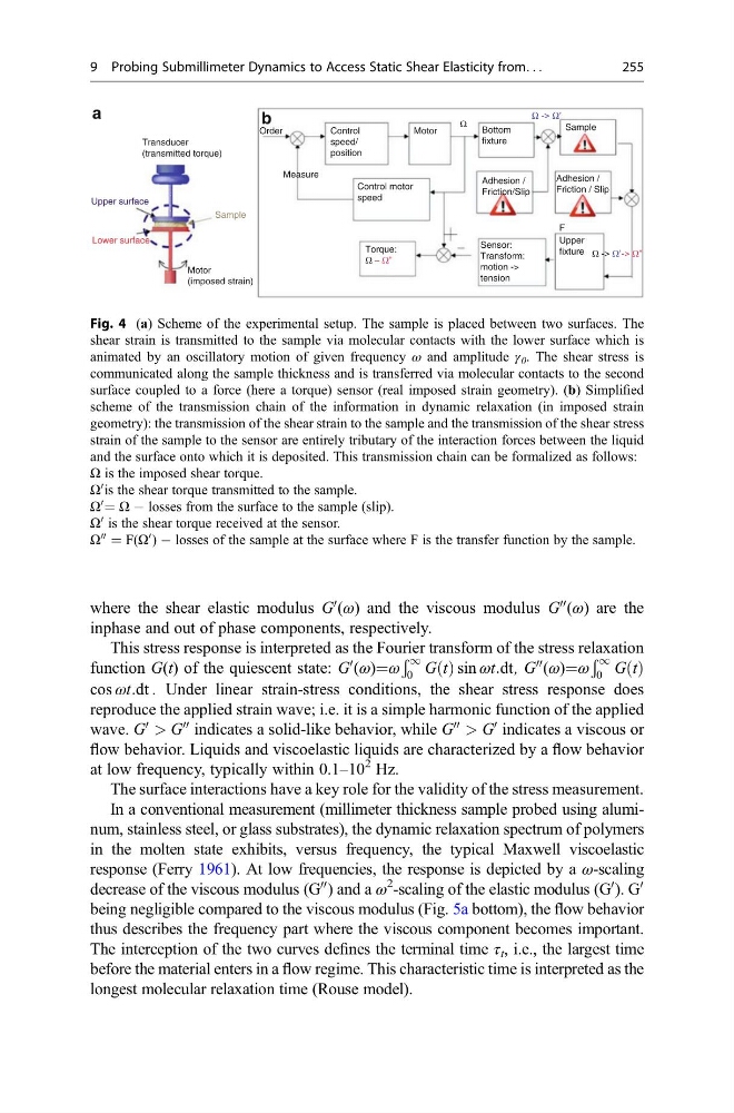
Fig. 4 (a) Scheme of the experimental setup. The sample is placed between two surfaces. The
shear strain is transmitted to the sample via molecular contacts with the lower surface which is
animated by an oscillatory motion of given frequency ω and amplitude γ 0 . The shear stress is
communicated along the sample thickness and is transferred via molecular contacts to the second
surface coupled to a force (here a torque) sensor (real imposed strain geometry). (b) Simplified
scheme of the transmission chain of the information in dynamic relaxation (in imposed strain
geometry): the transmission of the shear strain to the sample and the transmission of the shear stress
strain of the sample to the sensor are entirely tributary of the interaction forces between the liquid
and the surface onto which it is deposited. This transmission chain can be formalized as follows:
Ω is the imposed shear torque.
Ω
0 is the shear torque transmitted to the sample.
Ω
0 = Ω À losses from the surface to the sample (slip).
Ω
0 is the shear torque received at the sensor.
Ω
00 = F(Ω
0 ) À losses of the sample at the surface where F is the transfer function by the sample.
9 Probing Submillimeter Dynamics to Access Static Shear Elasticity from. . .
255
0 (ω) and the viscous modulus G
00 (ω) are the
inphase and out of phase components, respectively.
This stress response is interpreted as the Fourier transform of the stress relaxation
function G(t) of the quiescent state: G
0 (ω)=ω
Ð 1
0 G t
ð Þ sin ωt:dt, G
00 (ω)=ω
Ð 1
0 G t
ð Þ
cos ωt:dt . Under linear strain-stress conditions, the shear stress response does
reproduce the applied strain wave; i.e. it is a simple harmonic function of the applied
wave. G
0
> G
00 indicates a solid-like behavior, while G
00
> G
0 indicates a viscous or
flow behavior. Liquids and viscoelastic liquids are characterized by a flow behavior
at low frequency, typically within 0.1–10
2 Hz.
The surface interactions have a key role for the validity of the stress measurement.
In a conventional measurement (millimeter thickness sample probed using aluminum, stainless steel, or glass substrates), the dynamic relaxation spectrum of polymers
in the molten state exhibits, versus frequency, the typical Maxwell viscoelastic
response (Ferry 1961). At low frequencies, the response is depicted by a ω-scaling
decrease of the viscous modulus (G
00 ) and a ω
2
-scaling of the elastic modulus (G
0 ). G
0
being negligible compared to the viscous modulus (Fig. 5a bottom), the flow behavior
thus describes the frequency part where the viscous component becomes important.
The interception of the two curves defines the terminal time τ t , i.e., the largest time
before the material enters in a flow regime. This characteristic time is interpreted as the
longest molecular relaxation time (Rouse model).
Transducer
(transmitted torque)
Upper surface
Lower surface
Sample
Measure
Control
speed/
position
Control motor
speed
Motor
Bottom
fixture
Adhesion /
Friction/Slip
Adhesion /
Friction / Slip
Upper
fixture
F
Sensor:
Transform:
motion ->
tension
Torque:
Ω − Ω”
Ω -> Ω’-> Ω”
Ω
Sample
Order
a
b
Motor
(imposed strain)
Ω -> Ω’
Fig. 4 (a) Scheme of the experimental setup. The sample is placed between two surfaces. The
shear strain is transmitted to the sample via molecular contacts with the lower surface which is
animated by an oscillatory motion of given frequency ω and amplitude γ 0 . The shear stress is
communicated along the sample thickness and is transferred via molecular contacts to the second
surface coupled to a force (here a torque) sensor (real imposed strain geometry). (b) Simplified
scheme of the transmission chain of the information in dynamic relaxation (in imposed strain
geometry): the transmission of the shear strain to the sample and the transmission of the shear stress
strain of the sample to the sensor are entirely tributary of the interaction forces between the liquid
and the surface onto which it is deposited. This transmission chain can be formalized as follows:
Ω is the imposed shear torque.
Ω
0 is the shear torque transmitted to the sample.
Ω
0 = Ω À losses from the surface to the sample (slip).
Ω
0 is the shear torque received at the sensor.
Ω
00 = F(Ω
0 ) À losses of the sample at the surface where F is the transfer function by the sample.
9 Probing Submillimeter Dynamics to Access Static Shear Elasticity from. . .
255