

(i.e. same D, but different R) [19]. In this case, the short time would correspond to the
CO 2 molecules desorbing from the smallest crystals, while larger crystals would be
characterised by slower time constants.
The partial loading experiment is a very useful tool to resolve unequivocally what
the actual time constant of this sample is. By imposing a time constant on the system
and comparing not only the response at different flowrates but also at different
equilibration times, the experiments contain significant additional information that
constrains the fit to the point that one can reach a conclusion as to whether one has a
distribution of time constants or a main time constant that matches correctly all the
cases.
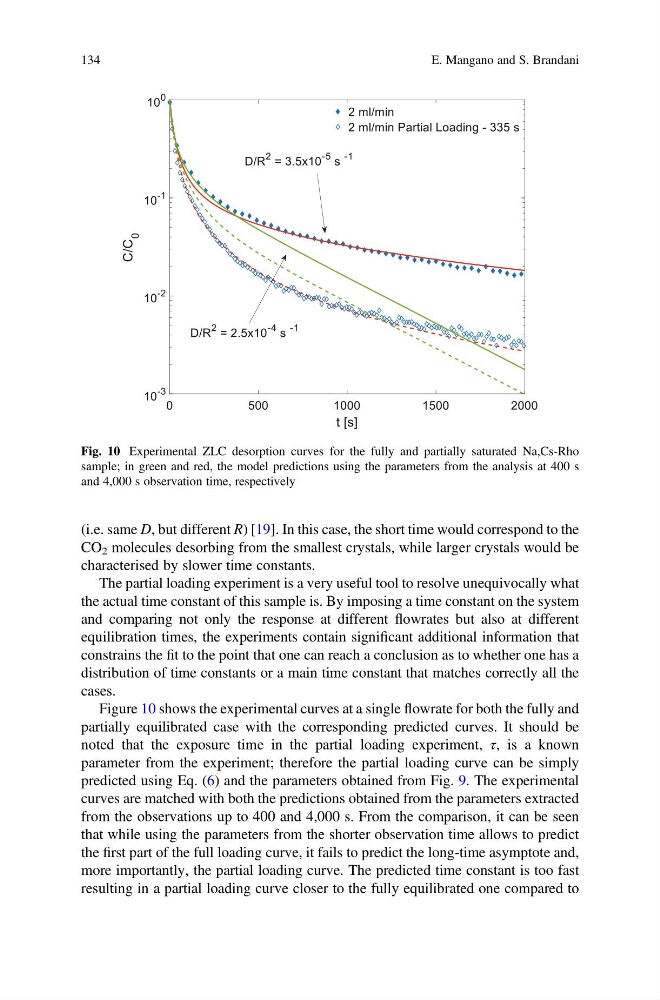
Figure 10 shows the experimental curves at a single flowrate for both the fully and
partially equilibrated case with the corresponding predicted curves. It should be
noted that the exposure time in the partial loading experiment, τ, is a known
parameter from the experiment; therefore the partial loading curve can be simply
predicted using Eq. (6) and the parameters obtained from Fig. 9. The experimental
curves are matched with both the predictions obtained from the parameters extracted
from the observations up to 400 and 4,000 s. From the comparison, it can be seen
that while using the parameters from the shorter observation time allows to predict
the first part of the full loading curve, it fails to predict the long-time asymptote and,
more importantly, the partial loading curve. The predicted time constant is too fast
resulting in a partial loading curve closer to the fully equilibrated one compared to
Fig. 10 Experimental ZLC desorption curves for the fully and partially saturated Na,Cs-Rho
sample; in green and red, the model predictions using the parameters from the analysis at 400 s
and 4,000 s observation time, respectively
134
E. Mangano and S. Brandani
CO 2 molecules desorbing from the smallest crystals, while larger crystals would be
characterised by slower time constants.
The partial loading experiment is a very useful tool to resolve unequivocally what
the actual time constant of this sample is. By imposing a time constant on the system
and comparing not only the response at different flowrates but also at different
equilibration times, the experiments contain significant additional information that
constrains the fit to the point that one can reach a conclusion as to whether one has a
distribution of time constants or a main time constant that matches correctly all the
cases.
Figure 10 shows the experimental curves at a single flowrate for both the fully and
partially equilibrated case with the corresponding predicted curves. It should be
noted that the exposure time in the partial loading experiment, τ, is a known
parameter from the experiment; therefore the partial loading curve can be simply
predicted using Eq. (6) and the parameters obtained from Fig. 9. The experimental
curves are matched with both the predictions obtained from the parameters extracted
from the observations up to 400 and 4,000 s. From the comparison, it can be seen
that while using the parameters from the shorter observation time allows to predict
the first part of the full loading curve, it fails to predict the long-time asymptote and,
more importantly, the partial loading curve. The predicted time constant is too fast
resulting in a partial loading curve closer to the fully equilibrated one compared to
Fig. 10 Experimental ZLC desorption curves for the fully and partially saturated Na,Cs-Rho
sample; in green and red, the model predictions using the parameters from the analysis at 400 s
and 4,000 s observation time, respectively
134
E. Mangano and S. Brandani