

Chapter II
Extreme Events
16
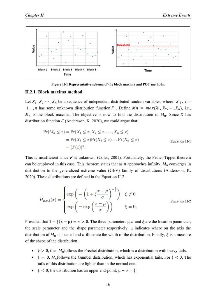
Figure II-1 Representative schema of the block maxima and POT methods.
II.2.1. Block maxima method
Let í µí± 1 , í µí± 2 , ⋯ , í µí± í µí± be a sequence of independent distributed random variables, where í µí± í µí± , í µí± =
1 … , í µí± has some unknown distribution function í µí°¹ . Define í µí±í µí± = í µí±í µí±í µí±¥{í µí± 1 , í µí± 2 , ⋯ , í µí± í µí± }, i.e.,
í µí± í µí± is the block maxima. The objective is now to find the distribution of í µí± í µí± . Since í µí± has
distribution function í µí°¹ (Andersson, K. 2020), we could argue that:
Equation II-1
This is insufficient since í µí°¹ is unknown, (Coles, 2001). Fortunately, the Fisher-Tippet theorem
can be employed in this case. This theorem states that as í µí± approaches infinity, í µí±ₙ converges in
distribution to the generalized extreme value (GEV) family of distributions (Andersson, K.
2020). These distributions are defined in the Equation II-2
Equation II-2
Provided that 1 + í µí¼(í µí±¥ − µ) = í µí¼ > 0. The three parameters µ, í µí¼ and í µí¼ are the location parameter,
the scale parameter and the shape parameter respectively. µ indicates where on the axis the
distribution of í µí± í µí± is located and í µí¼ illustrate the width of the distribution. Finally, í µí¼ is a measure
of the shape of the distribution.
• í µí¼ > 0, then í µí± í µí± follows the Fréchet distribution, which is a distribution with heavy tails.
• í µí¼ = 0, í µí± í µí± follows the Gumbel distribution, which has exponential tails. For í µí¼ < 0. The
tails of this distribution are lighter than in the normal one.
• í µí¼ < 0, the distribution has an upper end-point; µ − í µí¼ = í µí¼
Extreme Events
16
Figure II-1 Representative schema of the block maxima and POT methods.
II.2.1. Block maxima method
Let í µí± 1 , í µí± 2 , ⋯ , í µí± í µí± be a sequence of independent distributed random variables, where í µí± í µí± , í µí± =
1 … , í µí± has some unknown distribution function í µí°¹ . Define í µí±í µí± = í µí±í µí±í µí±¥{í µí± 1 , í µí± 2 , ⋯ , í µí± í µí± }, i.e.,
í µí± í µí± is the block maxima. The objective is now to find the distribution of í µí± í µí± . Since í µí± has
distribution function í µí°¹ (Andersson, K. 2020), we could argue that:
Equation II-1
This is insufficient since í µí°¹ is unknown, (Coles, 2001). Fortunately, the Fisher-Tippet theorem
can be employed in this case. This theorem states that as í µí± approaches infinity, í µí±ₙ converges in
distribution to the generalized extreme value (GEV) family of distributions (Andersson, K.
2020). These distributions are defined in the Equation II-2
Equation II-2
Provided that 1 + í µí¼(í µí±¥ − µ) = í µí¼ > 0. The three parameters µ, í µí¼ and í µí¼ are the location parameter,
the scale parameter and the shape parameter respectively. µ indicates where on the axis the
distribution of í µí± í µí± is located and í µí¼ illustrate the width of the distribution. Finally, í µí¼ is a measure
of the shape of the distribution.
• í µí¼ > 0, then í µí± í µí± follows the Fréchet distribution, which is a distribution with heavy tails.
• í µí¼ = 0, í µí± í µí± follows the Gumbel distribution, which has exponential tails. For í µí¼ < 0. The
tails of this distribution are lighter than in the normal one.
• í µí¼ < 0, the distribution has an upper end-point; µ − í µí¼ = í µí¼