

Chapter VII
Wave flume
92
í µí¼
2 = í µí±í µí± tanh(í µí±ℎ)
Equation VII-26
For a fixed period and a constant water depth, there is only one í µí± that satisfies Equation VII-26;
This value is determined by employing an iterative process (Table VII-2) to solve the equation.
Table VII-2 Iterative process for solving the dispersion equation.
For each period of range do.
1. Calculate the angular frequency í µí¼ for the period.
2. Choose an initial value for k.
3. Calculate the angular frequency í µí¼ ̅ corresponding to the value of k.
4. Evaluate the difference í µí¼
2 − í µí¼ ̅
2
.
5. If the difference is greater than the desired tolerance, increment k by STEP and go to
step3.
6. Else, save the value of k as the wave number of the considered period and go to the next
period (go to step1).
The STEP is evaluated by í µí±í µí±í µí°¸í µí± = í µí±í µí±í µí±í µí±í µí±í µí±í µí±í µí±í µí±í µí± ×
í µí±í µí±
í µí±(í µí¼ 2 )
|
í µí±=í µí±í µí±¢í µí±í µí±í µí±í µí±í µí±¡ í µí±£í µí±í µí±í µí±¢í µí± í µí±í µí± í µí±
. It’s clear from the
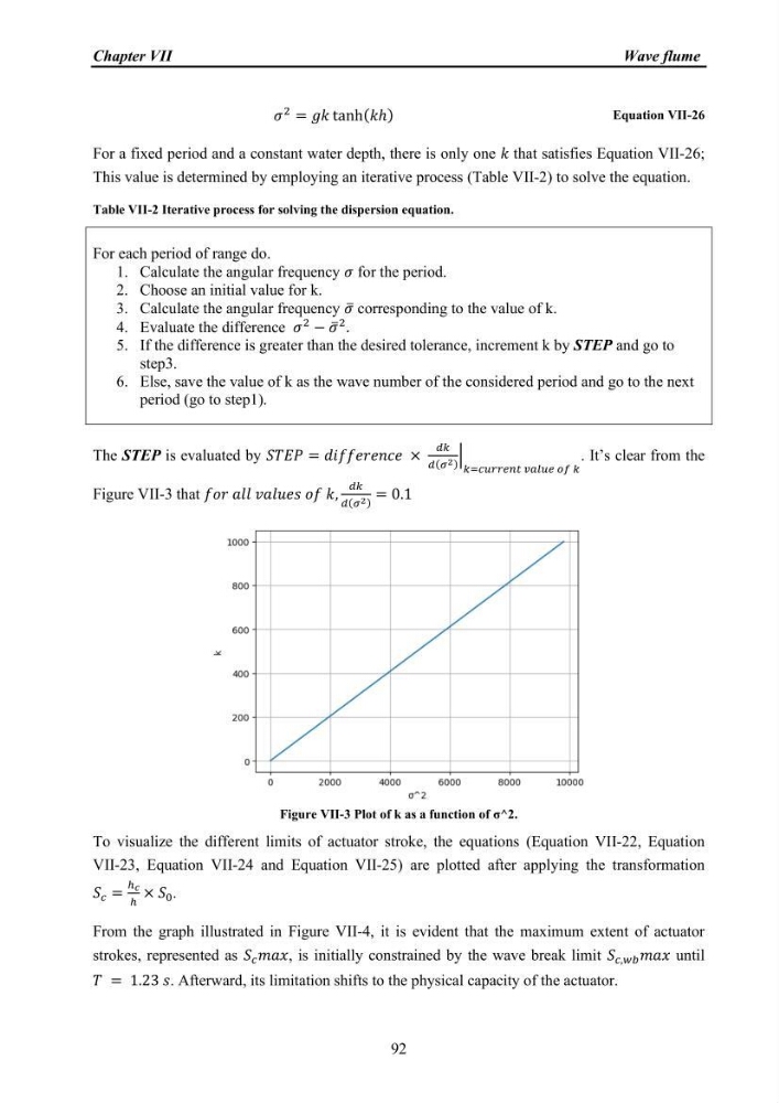
Figure VII-3 that í µí±í µí±í µí± í µí±í µí±í µí± í µí±£í µí±í µí±í µí±¢í µí±í µí± í µí±í µí± í µí±,
í µí±í µí±
í µí±(í µí¼ 2 )
= 0.1
Figure VII-3 Plot of k as a function of σ^2.
To visualize the different limits of actuator stroke, the equations (Equation VII-22, Equation
VII-23, Equation VII-24 and Equation VII-25) are plotted after applying the transformation
í µí± í µí± =
ℎ í µí±
ℎ
× í µí± 0 .
From the graph illustrated in Figure VII-4, it is evident that the maximum extent of actuator
strokes, represented as í µí± í µí± í µí±í µí±í µí±¥, is initially constrained by the wave break limit í µí± í µí±,í µí±¤í µí± í µí±í µí±í µí±¥ until
í µí± = 1.23 í µí± . Afterward, its limitation shifts to the physical capacity of the actuator.
Wave flume
92
í µí¼
2 = í µí±í µí± tanh(í µí±ℎ)
Equation VII-26
For a fixed period and a constant water depth, there is only one í µí± that satisfies Equation VII-26;
This value is determined by employing an iterative process (Table VII-2) to solve the equation.
Table VII-2 Iterative process for solving the dispersion equation.
For each period of range do.
1. Calculate the angular frequency í µí¼ for the period.
2. Choose an initial value for k.
3. Calculate the angular frequency í µí¼ ̅ corresponding to the value of k.
4. Evaluate the difference í µí¼
2 − í µí¼ ̅
2
.
5. If the difference is greater than the desired tolerance, increment k by STEP and go to
step3.
6. Else, save the value of k as the wave number of the considered period and go to the next
period (go to step1).
The STEP is evaluated by í µí±í µí±í µí°¸í µí± = í µí±í µí±í µí±í µí±í µí±í µí±í µí±í µí±í µí±í µí± ×
í µí±í µí±
í µí±(í µí¼ 2 )
|
í µí±=í µí±í µí±¢í µí±í µí±í µí±í µí±í µí±¡ í µí±£í µí±í µí±í µí±¢í µí± í µí±í µí± í µí±
. It’s clear from the
Figure VII-3 that í µí±í µí±í µí± í µí±í µí±í µí± í µí±£í µí±í µí±í µí±¢í µí±í µí± í µí±í µí± í µí±,
í µí±í µí±
í µí±(í µí¼ 2 )
= 0.1
Figure VII-3 Plot of k as a function of σ^2.
To visualize the different limits of actuator stroke, the equations (Equation VII-22, Equation
VII-23, Equation VII-24 and Equation VII-25) are plotted after applying the transformation
í µí± í µí± =
ℎ í µí±
ℎ
× í µí± 0 .
From the graph illustrated in Figure VII-4, it is evident that the maximum extent of actuator
strokes, represented as í µí± í µí± í µí±í µí±í µí±¥, is initially constrained by the wave break limit í µí± í µí±,í µí±¤í µí± í µí±í µí±í µí±¥ until
í µí± = 1.23 í µí± . Afterward, its limitation shifts to the physical capacity of the actuator.