

Chapter VII
Wave flume
91
First, we need to assess the wave generation capability of the flume. According to the linear
water wave theory. We can then determine the maximum expected wave height for each wave
period within the specified range. However, this assessment is subject to certain constraints that
affect the system. Therefore, the following limits need to be considered.
VII.3.1. Wave Break Limit
If the wave height exceeds the limit (
í µí°»
í µí°¿
<
1
7
), the wave will not maintain a regular shape and is
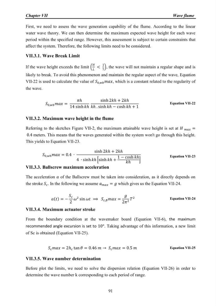
likely to break. To avoid this phenomenon and maintain the regular aspect of the wave, Equation
VII-22 is used to calculate the value of í µí± 0,í µí±¤í µí± í µí±í µí±í µí±¥, which is a constant related to the regularity of
the wave.
í µí± 0,í µí±¤í µí± í µí±í µí±í µí±¥ =
í µí¼ℎ
14 sinh í µí±ℎ
sinh 2í µí±ℎ + 2í µí±ℎ
í µí±ℎ . sinh í µí±ℎ − cosh í µí±ℎ + 1
Equation VII-22
VII.3.2. Maximum wave height in the flume
Referring to the sketches Figure VII-2, the maximum attainable wave height is set at í µí°» í µí±í µí±í µí±¥ =
0.4 meters. This means that the waves generated within the system won't go through this height.
This yields to Equation VII-23.
í µí± 0,í µí±¤ℎ í µí±í µí±í µí±¥ = 0.4 ∙
sinh 2í µí±ℎ + 2í µí±ℎ
4 ∙ sinh í µí±ℎ [sinh í µí±ℎ +
1 − cosh í µí±ℎ
í µí±ℎ
]
Equation VII-23
VII.3.3. Ballscrew maximum acceleration
The acceleration í µí± of the Ballscrew must be taken into consideration, as it directly depends on
the stroke í µí± í µí± . In the following we assume í µí± í µí±í µí±í µí±¥ = í µí± which gives us the Equation VII-24.
í µí±(í µí±¡) = −
í µí± í µí±
2
í µí¼
2 sin í µí¼í µí±¡ ⟹ í µí± í µí±,í µí°µ í µí±í µí±í µí±¥ =
í µí±
2í µí¼ 2 í µí±
2
Equation VII-24
VII.3.4. Maximum actuator stroke
From the boundary condition at the wavemaker board (Equation VII-6), the maximum
recommended angle excursion is set to 10°. Taking advantage of this information, a new limit
of Sc is obtained (Equation VII-25).
í µí± í µí± í µí±í µí±í µí±¥ = 2ℎ í µí± tan í µí¼ = 0.46 í µí± → í µí± í µí± í µí±í µí±í µí±¥ = 0.5 í µí±
Equation VII-25
VII.3.5. Wave number determination
Before plot the limits, we need to solve the dispersion relation (Equation VII-26) in order to
determine the wave number k corresponding to each period of range.
Wave flume
91
First, we need to assess the wave generation capability of the flume. According to the linear
water wave theory. We can then determine the maximum expected wave height for each wave
period within the specified range. However, this assessment is subject to certain constraints that
affect the system. Therefore, the following limits need to be considered.
VII.3.1. Wave Break Limit
If the wave height exceeds the limit (
í µí°»
í µí°¿
<
1
7
), the wave will not maintain a regular shape and is
likely to break. To avoid this phenomenon and maintain the regular aspect of the wave, Equation
VII-22 is used to calculate the value of í µí± 0,í µí±¤í µí± í µí±í µí±í µí±¥, which is a constant related to the regularity of
the wave.
í µí± 0,í µí±¤í µí± í µí±í µí±í µí±¥ =
í µí¼ℎ
14 sinh í µí±ℎ
sinh 2í µí±ℎ + 2í µí±ℎ
í µí±ℎ . sinh í µí±ℎ − cosh í µí±ℎ + 1
Equation VII-22
VII.3.2. Maximum wave height in the flume
Referring to the sketches Figure VII-2, the maximum attainable wave height is set at í µí°» í µí±í µí±í µí±¥ =
0.4 meters. This means that the waves generated within the system won't go through this height.
This yields to Equation VII-23.
í µí± 0,í µí±¤ℎ í µí±í µí±í µí±¥ = 0.4 ∙
sinh 2í µí±ℎ + 2í µí±ℎ
4 ∙ sinh í µí±ℎ [sinh í µí±ℎ +
1 − cosh í µí±ℎ
í µí±ℎ
]
Equation VII-23
VII.3.3. Ballscrew maximum acceleration
The acceleration í µí± of the Ballscrew must be taken into consideration, as it directly depends on
the stroke í µí± í µí± . In the following we assume í µí± í µí±í µí±í µí±¥ = í µí± which gives us the Equation VII-24.
í µí±(í µí±¡) = −
í µí± í µí±
2
í µí¼
2 sin í µí¼í µí±¡ ⟹ í µí± í µí±,í µí°µ í µí±í µí±í µí±¥ =
í µí±
2í µí¼ 2 í µí±
2
Equation VII-24
VII.3.4. Maximum actuator stroke
From the boundary condition at the wavemaker board (Equation VII-6), the maximum
recommended angle excursion is set to 10°. Taking advantage of this information, a new limit
of Sc is obtained (Equation VII-25).
í µí± í µí± í µí±í µí±í µí±¥ = 2ℎ í µí± tan í µí¼ = 0.46 í µí± → í µí± í µí± í µí±í µí±í µí±¥ = 0.5 í µí±
Equation VII-25
VII.3.5. Wave number determination
Before plot the limits, we need to solve the dispersion relation (Equation VII-26) in order to
determine the wave number k corresponding to each period of range.