

200
Chapter 4
1.0 \
0.8
\
0.6
0.5
0.4
0.3
0.2
0.1
.. ~
0 1 2 3
4 5 6 7 8 9 10
11
Time, Thousands of hours
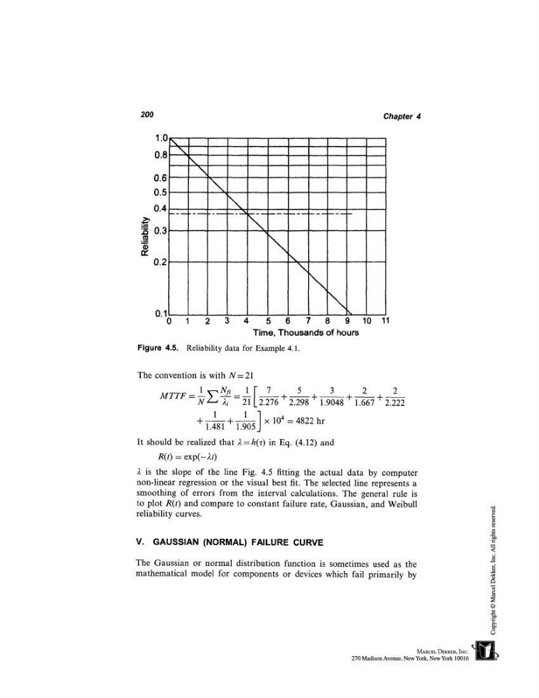
Figure 4.5. Reliability data for Example 4.1.
The convention is with N= 21
MTTF= l__s-.,Nfi_
1 [ 7
5
3
2
2
U z-’ 2i 21,.2.~ + 2.---~+ 1.-~0~ + 1.-~ -t 2.222
+~+
x 104=4822hr
It should be realized that 2=h(z) in Eq. (4.12)
R(t) = exp(-2t)
2 is the slope of the line Fig. 4.5 fitting the actual data by computer
non-linear regression or the visual best fit. The selected line represents a
smoothing of errors from the interval calculations. The general rule is
to plot R(t) and compare to constant failure rate, Gaussian, and Weibull
reliability curves.
V. GAUSSIAN (NORMAL) FAILURE CURVE
The Gaussian or normal distribution function is sometimes used as the
mathematical model for components or devices which fail primarily by
Chapter 4
1.0 \
0.8
\
0.6
0.5
0.4
0.3
0.2
0.1
.. ~
0 1 2 3
4 5 6 7 8 9 10
11
Time, Thousands of hours
Figure 4.5. Reliability data for Example 4.1.
The convention is with N= 21
MTTF= l__s-.,Nfi_
1 [ 7
5
3
2
2
U z-’ 2i 21,.2.~ + 2.---~+ 1.-~0~ + 1.-~ -t 2.222
+~+
x 104=4822hr
It should be realized that 2=h(z) in Eq. (4.12)
R(t) = exp(-2t)
2 is the slope of the line Fig. 4.5 fitting the actual data by computer
non-linear regression or the visual best fit. The selected line represents a
smoothing of errors from the interval calculations. The general rule is
to plot R(t) and compare to constant failure rate, Gaussian, and Weibull
reliability curves.
V. GAUSSIAN (NORMAL) FAILURE CURVE
The Gaussian or normal distribution function is sometimes used as the
mathematical model for components or devices which fail primarily by