

6.3 Axisymmetric Hertz Problem
57
(k 1 + k 2 )
(S)
p(ξ, η)dξ dη
(x − ξ) 2 + (y − η) 2
= F 2 (x, y) − F 1 (x, y) + δ,
(6.8)
where
k 1 =
1 − ν 2
1
πE 1
, k 2 =
1 − ν 2
2
πE 2
, δ = A 2 − A 1 .
(6.9)
We shall note that the constant value δ physically means the approach of infinitely
distanced points of the adjoining bodies as a result of their compression.
6.3 Axisymmetric Hertz Problem
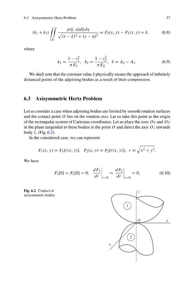
Let us consider a case when adjoining bodies are limited by smooth rotation surfaces
and the contact point O lies on the rotation axis. Let us take this point as the origin
of the rectangular system of Cartesian coordinates. Let us place the axes Ox and Oy
in the plane tangential to these bodies in the point O and direct the axis Oz inwards
body 1, (Fig. 6.2).
In the considered case, we can represent
F 1 (x, y) = F 1 [r(x, y)], F 2 (x, y) = F 2 [r(x, y)]; r =
x 2 + y 2 .
We have
F 1 [0] = F 2 [0] = 0;
dF 1
dr
r=0
=
dF 2
dr
r=0
= 0.
(6.10)
Fig. 6.2 Contact of
axisymmetric bodies
1
O
2
y
x
z
57
(k 1 + k 2 )
(S)
p(ξ, η)dξ dη
(x − ξ) 2 + (y − η) 2
= F 2 (x, y) − F 1 (x, y) + δ,
(6.8)
where
k 1 =
1 − ν 2
1
πE 1
, k 2 =
1 − ν 2
2
πE 2
, δ = A 2 − A 1 .
(6.9)
We shall note that the constant value δ physically means the approach of infinitely
distanced points of the adjoining bodies as a result of their compression.
6.3 Axisymmetric Hertz Problem
Let us consider a case when adjoining bodies are limited by smooth rotation surfaces
and the contact point O lies on the rotation axis. Let us take this point as the origin
of the rectangular system of Cartesian coordinates. Let us place the axes Ox and Oy
in the plane tangential to these bodies in the point O and direct the axis Oz inwards
body 1, (Fig. 6.2).
In the considered case, we can represent
F 1 (x, y) = F 1 [r(x, y)], F 2 (x, y) = F 2 [r(x, y)]; r =
x 2 + y 2 .
We have
F 1 [0] = F 2 [0] = 0;
dF 1
dr
r=0
=
dF 2
dr
r=0
= 0.
(6.10)
Fig. 6.2 Contact of
axisymmetric bodies
1
O
2
y
x
z