

412
32 On Boundary Value Problems of Inelastic Body Mechanics
32.3 An Example of Using the Birger Method
An example of solving the problem using the method of additional deformations was
implemented by Abdrakhmanov and Kozhobaev in the article [1]. For material with
linear plastic hardening, the authors use the method of successive approximations.
The main steps and results of the solution are described below.
32.3.1 The Initial Stage of the Process with Linear Hardening
Let us consider the uniaxial tension of a cylindrical rod of length l 0 and a crosssectional area of F beyond the yield strength under static loading with a constant
strain rate.
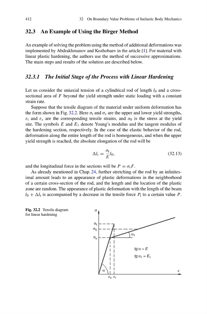
Suppose that the tensile diagram of the material under uniform deformation has
the form shown in Fig. 32.2. Here σ t and σ s are the upper and lower yield strengths,
ε t and ε s are the corresponding tensile strains, and σ 0 is the stress at the yield
site. The symbols E and E 1 denote Young’s modulus and the tangent modulus of
the hardening section, respectively. In the case of the elastic behavior of the rod,
deformation along the entire length of the rod is homogeneous, and when the upper
yield strength is reached, the absolute elongation of the rod will be
l t =
σ t
E
l 0 ,
(32.13)
and the longitudinal force in the sections will be P = σ t F.
As already mentioned in Chap. 24, further stretching of the rod by an infinitesimal amount leads to an appearance of plastic deformations in the neighborhood
of a certain cross-section of the rod, and the length and the location of the plastic
zone are random. The appearance of plastic deformation with the length of the beam
l 0 + l t is accompanied by a decrease in the tensile force P t to a certain value P .
Fig. 32.2 Tensile diagram
for linear hardening
σ
σ t
σ 0
ε S ε T
tg α = E
tg α 1 = E 1
ε
α
α 1
σ s
32 On Boundary Value Problems of Inelastic Body Mechanics
32.3 An Example of Using the Birger Method
An example of solving the problem using the method of additional deformations was
implemented by Abdrakhmanov and Kozhobaev in the article [1]. For material with
linear plastic hardening, the authors use the method of successive approximations.
The main steps and results of the solution are described below.
32.3.1 The Initial Stage of the Process with Linear Hardening
Let us consider the uniaxial tension of a cylindrical rod of length l 0 and a crosssectional area of F beyond the yield strength under static loading with a constant
strain rate.
Suppose that the tensile diagram of the material under uniform deformation has
the form shown in Fig. 32.2. Here σ t and σ s are the upper and lower yield strengths,
ε t and ε s are the corresponding tensile strains, and σ 0 is the stress at the yield
site. The symbols E and E 1 denote Young’s modulus and the tangent modulus of
the hardening section, respectively. In the case of the elastic behavior of the rod,
deformation along the entire length of the rod is homogeneous, and when the upper
yield strength is reached, the absolute elongation of the rod will be
l t =
σ t
E
l 0 ,
(32.13)
and the longitudinal force in the sections will be P = σ t F.
As already mentioned in Chap. 24, further stretching of the rod by an infinitesimal amount leads to an appearance of plastic deformations in the neighborhood
of a certain cross-section of the rod, and the length and the location of the plastic
zone are random. The appearance of plastic deformation with the length of the beam
l 0 + l t is accompanied by a decrease in the tensile force P t to a certain value P .
Fig. 32.2 Tensile diagram
for linear hardening
σ
σ t
σ 0
ε S ε T
tg α = E
tg α 1 = E 1
ε
α
α 1
σ s