

26.3 Proportional Loading of an Opposite Sign
347
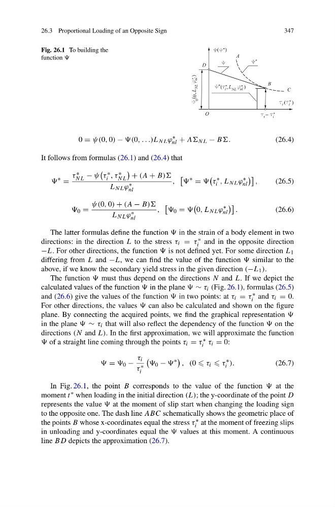
Fig. 26.1 To building the
function
0 = ψ(0, 0) − (0, . . .)L NL ϕ
∗
nl + AA NL − BB.
(26.4)
It follows from formulas (26.1) and (26.4) that
∗
=
τ ∗
NL − ψ
τ ∗
i , τ ∗
NL
+ (A + B))
L NL ϕ ∗
nl
,
∗
=
τ
∗
i , L NL ϕ
∗
nl
,
(26.5)
0 =
ψ(0, 0) + (A − B))
L NL ϕ ∗
nl
,
0 =
0, L NL ϕ
∗
nl
.
(26.6)
The latter formulas define the function in the strain of a body element in two
directions: in the direction L to the stress τ i = τ ∗
i and in the opposite direction
−L. For other directions, the function is not defined yet. For some direction L 1
differing from L and −L, we can find the value of the function similar to the
above, if we know the secondary yield stress in the given direction (−L 1 ).
The function must thus depend on the directions N and L. If we depict the
calculated values of the function in the plane ∼ τ i (Fig. 26.1), formulas (26.5)
and (26.6) give the values of the function in two points: at τ i = τ ∗
i and τ i = 0.
For other directions, the values can also be calculated and shown on the figure
plane. By connecting the acquired points, we find the graphical representation
in the plane ∼ τ i that will also reflect the dependency of the function on the
directions (N and L). In the first approximation, we will approximate the function
of a straight line coming through the points τ i = τ ∗
i τ i = 0:
= 0 −
τ i
τ ∗
i
0 −
∗
, (0 τ i τ
∗
i ).
(26.7)
In Fig. 26.1, the point B corresponds to the value of the function at the
moment t ∗ when loading in the initial direction (L); the y-coordinate of the point D
represents the value at the moment of slip start when changing the loading sign
to the opposite one. The dash line ABC schematically shows the geometric place of
the points B whose x-coordinates equal the stress τ ∗
i at the moment of freezing slips
in unloading and y-coordinates equal the values at this moment. A continuous
line BD depicts the approximation (26.7).
347
Fig. 26.1 To building the
function
0 = ψ(0, 0) − (0, . . .)L NL ϕ
∗
nl + AA NL − BB.
(26.4)
It follows from formulas (26.1) and (26.4) that
∗
=
τ ∗
NL − ψ
τ ∗
i , τ ∗
NL
+ (A + B))
L NL ϕ ∗
nl
,
∗
=
τ
∗
i , L NL ϕ
∗
nl
,
(26.5)
0 =
ψ(0, 0) + (A − B))
L NL ϕ ∗
nl
,
0 =
0, L NL ϕ
∗
nl
.
(26.6)
The latter formulas define the function in the strain of a body element in two
directions: in the direction L to the stress τ i = τ ∗
i and in the opposite direction
−L. For other directions, the function is not defined yet. For some direction L 1
differing from L and −L, we can find the value of the function similar to the
above, if we know the secondary yield stress in the given direction (−L 1 ).
The function must thus depend on the directions N and L. If we depict the
calculated values of the function in the plane ∼ τ i (Fig. 26.1), formulas (26.5)
and (26.6) give the values of the function in two points: at τ i = τ ∗
i and τ i = 0.
For other directions, the values can also be calculated and shown on the figure
plane. By connecting the acquired points, we find the graphical representation
in the plane ∼ τ i that will also reflect the dependency of the function on the
directions (N and L). In the first approximation, we will approximate the function
of a straight line coming through the points τ i = τ ∗
i τ i = 0:
= 0 −
τ i
τ ∗
i
0 −
∗
, (0 τ i τ
∗
i ).
(26.7)
In Fig. 26.1, the point B corresponds to the value of the function at the
moment t ∗ when loading in the initial direction (L); the y-coordinate of the point D
represents the value at the moment of slip start when changing the loading sign
to the opposite one. The dash line ABC schematically shows the geometric place of
the points B whose x-coordinates equal the stress τ ∗
i at the moment of freezing slips
in unloading and y-coordinates equal the values at this moment. A continuous
line BD depicts the approximation (26.7).