

306
20 Problem Setting
In the latter conditions, the stress tensor component τ νλ is an arbitrary set function
of time and is expressed through the known components of the stress tensor under
the formula:
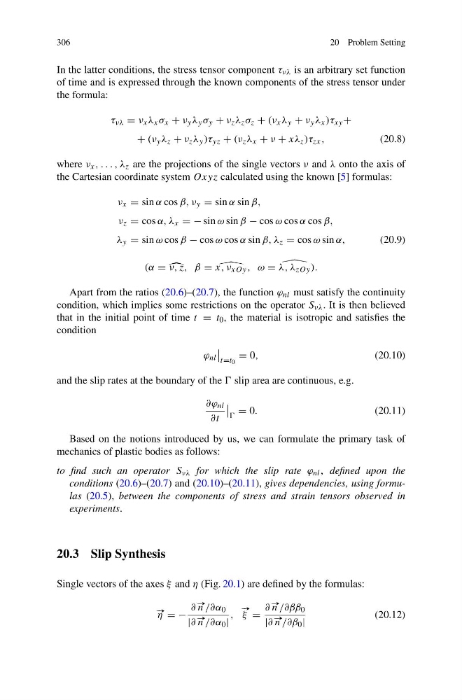
τ νλ = ν x λ x σ x + ν y λ y σ y + ν z λ z σ z + (ν x λ y + ν y λ x )τ xy +
+ (ν y λ z + ν z λ y )τ yz + (ν z λ x + ν + xλ z )τ zx ,
(20.8)
where ν x , . . . , λ z are the projections of the single vectors ν and λ onto the axis of
the Cartesian coordinate system Oxyz calculated using the known [5] formulas:
ν x = sin α cos β, ν y = sin α sin β,
ν z = cos α, λ x = − sin ω sin β − cos ω cos α cos β,
λ y = sin ω cos β − cos ω cos α sin β, λ z = cos ω sin α,
(20.9)
(α =
ν, z, β =
x, ν xOy , ω =
λ, λ zOy ).
Apart from the ratios (20.6)–(20.7), the function ϕ nl must satisfy the continuity
condition, which implies some restrictions on the operator S νλ . It is then believed
that in the initial point of time t = t 0 , the material is isotropic and satisfies the
condition
ϕ nl
t=t 0
= 0,
(20.10)
and the slip rates at the boundary of the slip area are continuous, e.g.
∂ϕ nl
∂t
= 0.
(20.11)
Based on the notions introduced by us, we can formulate the primary task of
mechanics of plastic bodies as follows:
to find such an operator S νλ for which the slip rate ϕ nl , defined upon the
conditions (20.6)–(20.7) and (20.10)–(20.11), gives dependencies, using formulas (20.5), between the components of stress and strain tensors observed in
experiments.
20.3 Slip Synthesis
Single vectors of the axes ξ and η (Fig. 20.1) are defined by the formulas:
#» η = −
∂ #» n /∂α 0
|∂ #» n /∂α 0 |
,
#»
ξ =
∂ #» n /∂ββ 0
|∂ #» n /∂β 0 |
(20.12)
20 Problem Setting
In the latter conditions, the stress tensor component τ νλ is an arbitrary set function
of time and is expressed through the known components of the stress tensor under
the formula:
τ νλ = ν x λ x σ x + ν y λ y σ y + ν z λ z σ z + (ν x λ y + ν y λ x )τ xy +
+ (ν y λ z + ν z λ y )τ yz + (ν z λ x + ν + xλ z )τ zx ,
(20.8)
where ν x , . . . , λ z are the projections of the single vectors ν and λ onto the axis of
the Cartesian coordinate system Oxyz calculated using the known [5] formulas:
ν x = sin α cos β, ν y = sin α sin β,
ν z = cos α, λ x = − sin ω sin β − cos ω cos α cos β,
λ y = sin ω cos β − cos ω cos α sin β, λ z = cos ω sin α,
(20.9)
(α =
ν, z, β =
x, ν xOy , ω =
λ, λ zOy ).
Apart from the ratios (20.6)–(20.7), the function ϕ nl must satisfy the continuity
condition, which implies some restrictions on the operator S νλ . It is then believed
that in the initial point of time t = t 0 , the material is isotropic and satisfies the
condition
ϕ nl
t=t 0
= 0,
(20.10)
and the slip rates at the boundary of the slip area are continuous, e.g.
∂ϕ nl
∂t
= 0.
(20.11)
Based on the notions introduced by us, we can formulate the primary task of
mechanics of plastic bodies as follows:
to find such an operator S νλ for which the slip rate ϕ nl , defined upon the
conditions (20.6)–(20.7) and (20.10)–(20.11), gives dependencies, using formulas (20.5), between the components of stress and strain tensors observed in
experiments.
20.3 Slip Synthesis
Single vectors of the axes ξ and η (Fig. 20.1) are defined by the formulas:
#» η = −
∂ #» n /∂α 0
|∂ #» n /∂α 0 |
,
#»
ξ =
∂ #» n /∂ββ 0
|∂ #» n /∂β 0 |
(20.12)