

280
18 Theories of Plastic Yield
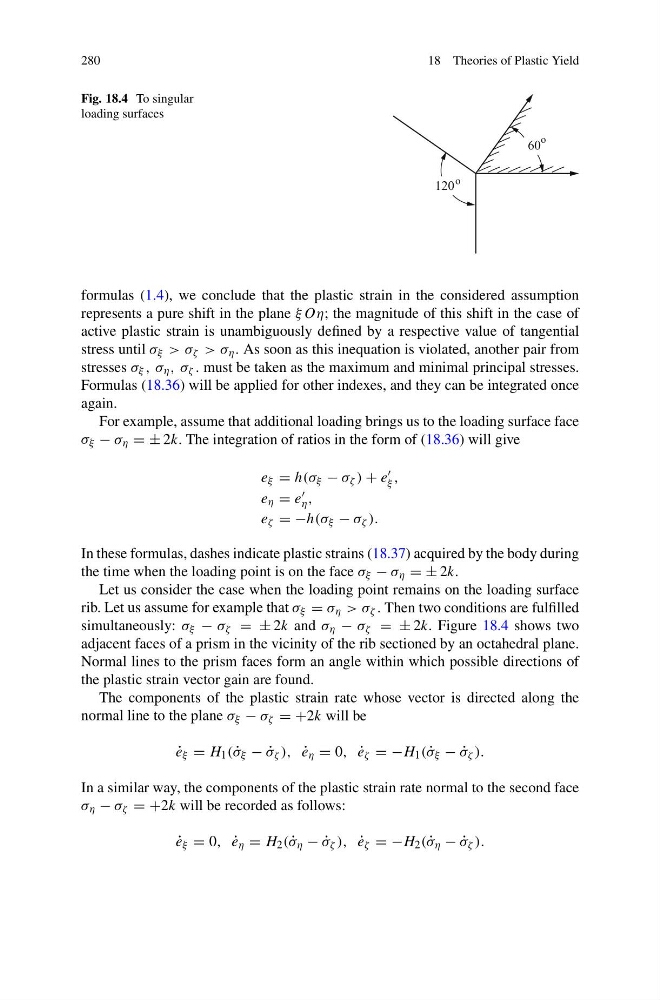
Fig. 18.4 To singular
loading surfaces
formulas (1.4), we conclude that the plastic strain in the considered assumption
represents a pure shift in the plane ξOη; the magnitude of this shift in the case of
active plastic strain is unambiguously defined by a respective value of tangential
stress until σ ξ > σ ζ > σ η . As soon as this inequation is violated, another pair from
stresses σ ξ , σ η , σ ζ . must be taken as the maximum and minimal principal stresses.
Formulas (18.36) will be applied for other indexes, and they can be integrated once
again.
For example, assume that additional loading brings us to the loading surface face
σ ξ − σ η = ± 2k. The integration of ratios in the form of (18.36) will give
e ξ = h(σ ξ − σ ζ ) + e
ξ ,
e η = e
η ,
e ζ = −h(σ ξ − σ ζ ).
In these formulas, dashes indicate plastic strains (18.37) acquired by the body during
the time when the loading point is on the face σ ξ − σ η = ± 2k.
Let us consider the case when the loading point remains on the loading surface
rib. Let us assume for example that σ ξ = σ η > σ ζ . Then two conditions are fulfilled
simultaneously: σ ξ − σ ζ = ± 2k and σ η − σ ζ = ± 2k. Figure 18.4 shows two
adjacent faces of a prism in the vicinity of the rib sectioned by an octahedral plane.
Normal lines to the prism faces form an angle within which possible directions of
the plastic strain vector gain are found.
The components of the plastic strain rate whose vector is directed along the
normal line to the plane σ ξ − σ ζ = +2k will be
˙
e ξ = H 1 ( ˙
σ ξ − ˙
σ ζ ), ˙
e η = 0, ˙
e ζ = −H 1 ( ˙
σ ξ − ˙
σ ζ ).
In a similar way, the components of the plastic strain rate normal to the second face
σ η − σ ζ = +2k will be recorded as follows:
˙
e ξ = 0, ˙
e η = H 2 ( ˙
σ η − ˙
σ ζ ), ˙
e ζ = −H 2 ( ˙
σ η − ˙
σ ζ ).
18 Theories of Plastic Yield
Fig. 18.4 To singular
loading surfaces
formulas (1.4), we conclude that the plastic strain in the considered assumption
represents a pure shift in the plane ξOη; the magnitude of this shift in the case of
active plastic strain is unambiguously defined by a respective value of tangential
stress until σ ξ > σ ζ > σ η . As soon as this inequation is violated, another pair from
stresses σ ξ , σ η , σ ζ . must be taken as the maximum and minimal principal stresses.
Formulas (18.36) will be applied for other indexes, and they can be integrated once
again.
For example, assume that additional loading brings us to the loading surface face
σ ξ − σ η = ± 2k. The integration of ratios in the form of (18.36) will give
e ξ = h(σ ξ − σ ζ ) + e
ξ ,
e η = e
η ,
e ζ = −h(σ ξ − σ ζ ).
In these formulas, dashes indicate plastic strains (18.37) acquired by the body during
the time when the loading point is on the face σ ξ − σ η = ± 2k.
Let us consider the case when the loading point remains on the loading surface
rib. Let us assume for example that σ ξ = σ η > σ ζ . Then two conditions are fulfilled
simultaneously: σ ξ − σ ζ = ± 2k and σ η − σ ζ = ± 2k. Figure 18.4 shows two
adjacent faces of a prism in the vicinity of the rib sectioned by an octahedral plane.
Normal lines to the prism faces form an angle within which possible directions of
the plastic strain vector gain are found.
The components of the plastic strain rate whose vector is directed along the
normal line to the plane σ ξ − σ ζ = +2k will be
˙
e ξ = H 1 ( ˙
σ ξ − ˙
σ ζ ), ˙
e η = 0, ˙
e ζ = −H 1 ( ˙
σ ξ − ˙
σ ζ ).
In a similar way, the components of the plastic strain rate normal to the second face
σ η − σ ζ = +2k will be recorded as follows:
˙
e ξ = 0, ˙
e η = H 2 ( ˙
σ η − ˙
σ ζ ), ˙
e ζ = −H 2 ( ˙
σ η − ˙
σ ζ ).