

14.5 Experimental Study of Elastic–Plastic Materials
189
the inner surface of the tube and turns zero on the outer surface. Due to a small size
of the component σ z as compared to three other components of stress, σ z = 0 is
adopted everywhere in the specimen body.
In this manner, in the case of complicated loading of a tubular specimen, an
arbitrary plane stressed state can be achieved. The axis z is the main axis of the
tensor state. It is substantial that each stress component depends on one force only,
and therefore, each component can be changed irrespective of each other.
The specimen strain will be represented by the components ε x , ε y abd γ xy . To
determine them experimentally, we must measure the elongation l of the working
part (l) of the specimen, the change of the radius R, as well as the angle (ϕ) of
turning of one fixed section of the tube relative to the other one distanced from the
first one by l 1 . Then,
ε x =
l
l
, ε y =
(2πR)
2πR
=
R
R
, γ xy =
Rϕ
l 1
.
(14.21)
The strain ε z can be determined by measuring the change in the tube wall thickness
or calculated using the formula
ε z = −ε x − ε y +
σ 0
3K
,
(14.22)
where K is the volumetric elasticity modulus defined by formula (1.17). Equation
(14.22) is a consequence of the first of formulas (1.16).
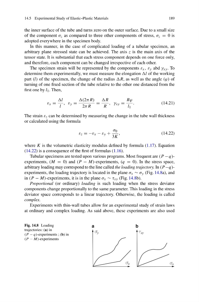
Tubular specimens are tested upon various programs. Most frequent are (P − q)experiments, (M = 0) and (P − M)-experiments, (q = 0). In the stress space,
arbitrary loading may correspond to the line called the loading trajectory. In (P −q)experiments, the loading trajectory is located in the plane σ x ∼ σ y (Fig. 14.8a), and
in (P − M)-experiments, it is in the plane σ x ∼ τ xy (Fig. 14.8b).
Proportional (or ordinary) loading is such loading when the stress deviator
components change proportionally to the same parameter. This loading in the stress
deviator space corresponds to a linear trajectory. Otherwise, the loading is called
complex.
Experiments with thin-wall tubes allow for an experimental study of strain laws
at ordinary and complex loading. As said above, these experiments are also used
Fig. 14.8 Loading
trajectories: (a) in
(P − q)-experiments ; (b) in
(P − M)-experiments
a
b
189
the inner surface of the tube and turns zero on the outer surface. Due to a small size
of the component σ z as compared to three other components of stress, σ z = 0 is
adopted everywhere in the specimen body.
In this manner, in the case of complicated loading of a tubular specimen, an
arbitrary plane stressed state can be achieved. The axis z is the main axis of the
tensor state. It is substantial that each stress component depends on one force only,
and therefore, each component can be changed irrespective of each other.
The specimen strain will be represented by the components ε x , ε y abd γ xy . To
determine them experimentally, we must measure the elongation l of the working
part (l) of the specimen, the change of the radius R, as well as the angle (ϕ) of
turning of one fixed section of the tube relative to the other one distanced from the
first one by l 1 . Then,
ε x =
l
l
, ε y =
(2πR)
2πR
=
R
R
, γ xy =
Rϕ
l 1
.
(14.21)
The strain ε z can be determined by measuring the change in the tube wall thickness
or calculated using the formula
ε z = −ε x − ε y +
σ 0
3K
,
(14.22)
where K is the volumetric elasticity modulus defined by formula (1.17). Equation
(14.22) is a consequence of the first of formulas (1.16).
Tubular specimens are tested upon various programs. Most frequent are (P − q)experiments, (M = 0) and (P − M)-experiments, (q = 0). In the stress space,
arbitrary loading may correspond to the line called the loading trajectory. In (P −q)experiments, the loading trajectory is located in the plane σ x ∼ σ y (Fig. 14.8a), and
in (P − M)-experiments, it is in the plane σ x ∼ τ xy (Fig. 14.8b).
Proportional (or ordinary) loading is such loading when the stress deviator
components change proportionally to the same parameter. This loading in the stress
deviator space corresponds to a linear trajectory. Otherwise, the loading is called
complex.
Experiments with thin-wall tubes allow for an experimental study of strain laws
at ordinary and complex loading. As said above, these experiments are also used
Fig. 14.8 Loading
trajectories: (a) in
(P − q)-experiments ; (b) in
(P − M)-experiments
a
b