

112
10 Mathematical Structural Imperfections
where the right part of the equation symbolically writes the sum of deductions of
the function N(z) in all special points a i of the area limited by the outline .
By equating the right parts of equations (10.25) and (10.26), we will obtain
1
2πi
+R
−R
N(ζ )dζ
ζ − z
=
1
2πi
C
N(ζ )dζ
ζ − z
− res N(a i ).
(10.27)
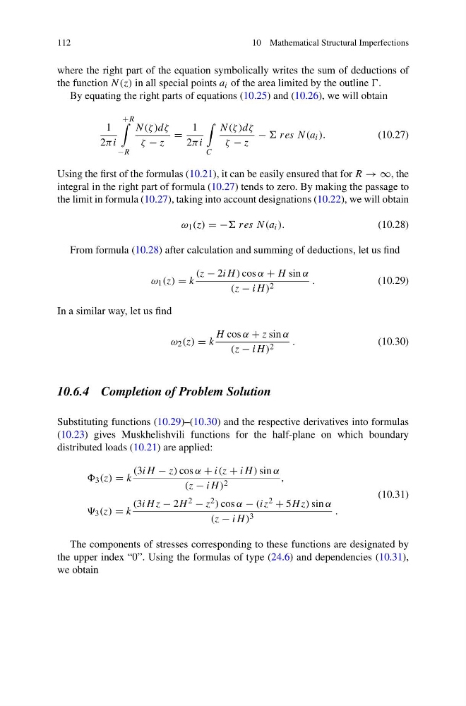
Using the first of the formulas (10.21), it can be easily ensured that for R → ∞, the
integral in the right part of formula (10.27) tends to zero. By making the passage to
the limit in formula (10.27), taking into account designations (10.22), we will obtain
ω 1 (z) = − res N(a i ).
(10.28)
From formula (10.28) after calculation and summing of deductions, let us find
ω 1 (z) = k
(z − 2iH ) cos α + H sin α
(z − iH ) 2
.
(10.29)
In a similar way, let us find
ω 2 (z) = k
H cos α + z sin α
(z − iH ) 2
.
(10.30)
10.6.4 Completion of Problem Solution
Substituting functions (10.29)–(10.30) and the respective derivatives into formulas
(10.23) gives Muskhelishvili functions for the half-plane on which boundary
distributed loads (10.21) are applied:
3 (z) = k
(3iH − z) cos α + i(z + iH ) sin α
(z − iH ) 2
,
3 (z) = k
(3iH z − 2H 2 − z 2 ) cos α − (iz 2 + 5H z) sin α
(z − iH ) 3
.
(10.31)
The components of stresses corresponding to these functions are designated by
the upper index “0”. Using the formulas of type (24.6) and dependencies (10.31),
we obtain
10 Mathematical Structural Imperfections
where the right part of the equation symbolically writes the sum of deductions of
the function N(z) in all special points a i of the area limited by the outline .
By equating the right parts of equations (10.25) and (10.26), we will obtain
1
2πi
+R
−R
N(ζ )dζ
ζ − z
=
1
2πi
C
N(ζ )dζ
ζ − z
− res N(a i ).
(10.27)
Using the first of the formulas (10.21), it can be easily ensured that for R → ∞, the
integral in the right part of formula (10.27) tends to zero. By making the passage to
the limit in formula (10.27), taking into account designations (10.22), we will obtain
ω 1 (z) = − res N(a i ).
(10.28)
From formula (10.28) after calculation and summing of deductions, let us find
ω 1 (z) = k
(z − 2iH ) cos α + H sin α
(z − iH ) 2
.
(10.29)
In a similar way, let us find
ω 2 (z) = k
H cos α + z sin α
(z − iH ) 2
.
(10.30)
10.6.4 Completion of Problem Solution
Substituting functions (10.29)–(10.30) and the respective derivatives into formulas
(10.23) gives Muskhelishvili functions for the half-plane on which boundary
distributed loads (10.21) are applied:
3 (z) = k
(3iH − z) cos α + i(z + iH ) sin α
(z − iH ) 2
,
3 (z) = k
(3iH z − 2H 2 − z 2 ) cos α − (iz 2 + 5H z) sin α
(z − iH ) 3
.
(10.31)
The components of stresses corresponding to these functions are designated by
the upper index “0”. Using the formulas of type (24.6) and dependencies (10.31),
we obtain